Lab 10: Grid Localization using Bayes Filter (simulation)

Objective

The objective of this lab was to set up the simulation environment and write the Bayes Filter.

Lab work

PreLab

For the pre-lab, I had to set up the simulator environment. This meant downloading the notebook and installing the dependencies in the venv. I did this, as well as the tasks of open and closed-loop control, in class.

Lab Tasks

Compute Control

The first step is to compute the robot’s motion based on the current and previous poses. These are the ideal motion of the car. The odometry model models motion as an initial rotation, a translation from the initial position to the final position, and a final rotation to get the final orientation. These motions are modeled with the following equations:

$$\delta_{rot1} = \text{atan2}(\bar{y}' - \bar{y},\ \bar{x}' - \bar{x}) - \bar{\theta}$$ $$\delta_{trans} = \sqrt{(\bar{y}' - \bar{y})^2 + (\bar{x}' - \bar{x})^2}$$ $$\delta_{rot2} = \bar{\theta}' - \bar{\theta} - \delta_{rot1}$$

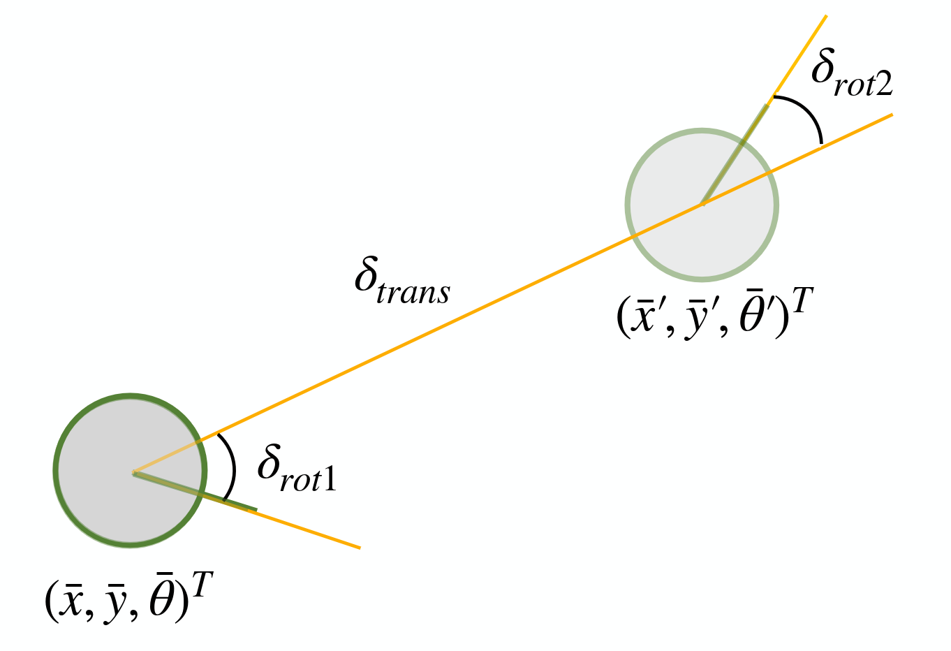
This is the code used to compute the motion:

def compute_control(cur_pose, prev_pose):
    """ Given the current and previous odometry poses, this function extracts
    the control information based on the odometry motion model.

    Args:
        cur_pose  ([Pose]): Current Pose
        prev_pose ([Pose]): Previous Pose 

    Returns:
        [delta_rot_1]: Rotation 1  (degrees)
        [delta_trans]: Translation (meters)
        [delta_rot_2]: Rotation 2  (degrees)
    """
    dx = cur_pose[0] - prev_pose[0]
    dy = cur_pose[1] - prev_pose[1]
    dang = cur_pose[2] - prev_pose[2]
    
    
    delta_rot_1 = mapper.normalize_angle(math.degrees(math.atan2(dy, dx)) - prev_pose[2])
    delta_trans = math.sqrt((dy)**2 + (dx)**2)
    delta_rot_2 = mapper.normalize_angle(dang - delta_rot_1)
    
    return delta_rot_1, delta_trans, delta_rot_2

Odometry Motion Model

With the ideal motion parameters computed, the next step is to compute the probability that the robot executed the computed motion based on its sensor readings. We use the odometry readings and the Gaussian function with the calculated ideal values and the odometry noise parameters to compute the probability of each motion step. The following math shows the steps:

$$\hat{\delta}_{rot1} = \text{atan2}(y' - y,\ x' - x) - \theta$$ $$\hat{\delta}_{trans} = \sqrt{(x' - x)^2 + (y' - y)^2}$$ $$\hat{\delta}_{rot2} = \theta' - \theta - \hat{\delta}_{rot1}$$ $$p_1 = \text{prob}(\delta_{rot1} - \hat{\delta}_{rot1},\ \alpha_1 \hat{\delta}_{rot1}^2 + \alpha_2 \hat{\delta}_{trans}^2)$$ $$p_2 = \text{prob}(\delta_{trans} - \hat{\delta}_{trans},\ \alpha_3 \hat{\delta}_{trans}^2 + \alpha_4 \hat{\delta}_{rot1}^2 + \alpha_4 \hat{\delta}_{rot2}^2)$$ $$p_3 = \text{prob}(\delta_{rot2} - \hat{\delta}_{rot2},\ \alpha_1 \hat{\delta}_{rot2}^2 + \alpha_2 \hat{\delta}_{trans}^2)$$ $$\text{return } p_1 \cdot p_2 \cdot p_3$$

And is implemented in the following code:

def odom_motion_model(cur_pose, prev_pose, u):
    """ Odometry Motion Model

    Args:
        cur_pose  ([Pose]): Current Pose
        prev_pose ([Pose]): Previous Pose
        (rot1, trans, rot2) (float, float, float): A tuple with control data in the format 
                                                   format (rot1, trans, rot2) with units (degrees, meters, degrees)


    Returns:
        prob [float]: Probability p(x'|x, u)
    """
    # Compute ideal motion
    delta_rot1_hat, delta_trans_hat, delta_rot2_hat = compute_control(cur_pose, prev_pose)

    # Actual odometry readings
    delta_rot1, delta_trans, delta_rot2 = u

    rot_sigma = loc.odom_rot_sigma
    trans_sigma = loc.odom_trans_sigma

    # Probabilities
    p1 = loc.gaussian(delta_rot1,  delta_rot1_hat,  rot_sigma)
    p2 = loc.gaussian(delta_trans, delta_trans_hat, trans_sigma)
    p3 = loc.gaussian(delta_rot2,  delta_rot2_hat,  rot_sigma)
    
    
    return p1 * p2 * p3

Prediction Step

With the odometry model complete, it is time to use it to update the Bayes filter beliefs. It loops over every possible state on the map twice, once for the current pose and once for the previous pose, and uses the odometry motion model to calculate the probability that the robot moved to that state based on the odometry readings. Each previous state’s contribution is weighted by the prior belief of that state and summed to form the new predicted belief. To save some performance, it skips the calculation for any previous state that was unlikely (less than 0.1%). This is implemented with the following code:

def prediction_step(cur_odom, prev_odom):
    """ Prediction step of the Bayes Filter.
    Update the probabilities in loc.bel_bar based on loc.bel from the previous time step and the odometry motion model.

    Args:
        cur_odom  ([Pose]): Current Pose
        prev_odom ([Pose]): Previous Pose
    """

    u = compute_control(cur_odom, prev_odom)

    for cx, cy, ca in np.ndindex(mapper.MAX_CELLS_X, mapper.MAX_CELLS_Y, mapper.MAX_CELLS_A):
        cur_pose = mapper.from_map(cx, cy, ca)

        bel_bar_sum = 0.0

        for px, py, pa in np.ndindex(mapper.MAX_CELLS_X, mapper.MAX_CELLS_Y, mapper.MAX_CELLS_A):
            # Skip small beliefs
            if loc.bel[px, py, pa] < 0.0001:
                continue

            prev_pose = mapper.from_map(px, py, pa)
            prob = odom_motion_model(cur_pose, prev_pose, u)
            bel_bar_sum += prob * loc.bel[px, py, pa]

        loc.bel_bar[cx, cy, ca] = bel_bar_sum

    # Normalize since skipped cells mean probabilities no longer sum to 1
    loc.bel = loc.bel / np.sum(loc.bel_bar)

Sensor Model

To get the pose, the robot stops in place and rotates 360° while taking measurements from the ToF sensor (18 in total). It then calculates the probability of the actual reading based on the expected measurement from the map using a Gaussian. This is the code to implement it:

def sensor_model(obs):
    """ This is the equivalent of p(z|x).


    Args:
        obs ([ndarray]): A 1D array consisting of the true observations for a specific robot pose in the map 

    Returns:
        [ndarray]: Returns a 1D array of size 18 (=loc.OBS_PER_CELL) with the likelihoods of each individual sensor measurement
    """
    prob_array = loc.gaussian(obs, loc.obs_range_data.flatten(), loc.sensor_sigma) #flatten the range data from 2D (18,1) array to 1D array
    return prob_array

Update Step

The update step loops through every pose on the map, runs the sensor model to compare the robot’s actual ToF readings against the precomputed expected readings for that cell, and multiplies the result by the prior belief from the prediction step. The beliefs are then normalized so they sum to 1. This is the code:

def update_step():
    """ Update step of the Bayes Filter.
    Update the probabilities in loc.bel based on loc.bel_bar and the sensor model.
    """
    for cx, cy, ca in np.ndindex(mapper.MAX_CELLS_X, mapper.MAX_CELLS_Y, mapper.MAX_CELLS_A):
        # get sensor model
        sens = sensor_model(mapper.get_views(cx, cy, ca))
        loc.bel[cx, cy, ca] = np.prod(sens) * loc.bel_bar[cx, cy, ca]

    #Normalize
    loc.bel /= np.sum(loc.bel)

Results

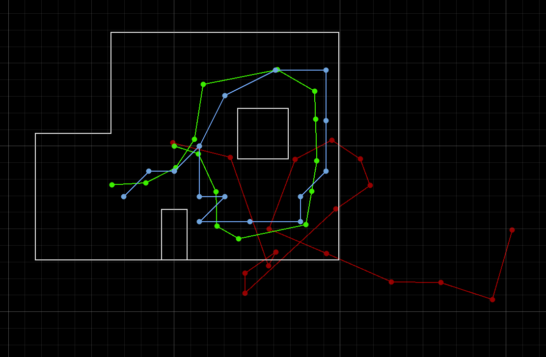
Below is the output of the simulator with the actual movement in green, the raw odometry in red, and the Bayes filter in blue. The odometry alone is not great at tracking; errors accumulate quickly and mean that very quickly the results are garbage. The Bayes filter, on the other hand, stays pretty consistent. It’s not perfect, but much better than the odometry alone.

Acknowledgements

For this lab, I referenced Henry Calderon and Aidan McNay’s lab write-ups from last year to see how other people implemented the functions. I used AI to convert my lab write-up from a Google Doc to Markdown with the correct formatting.