
Lab 11: Grid Localization using Bayes Filter (real)
Objective
The objective of this lab was to use the simulator with the robot to test whether the Bayes filter worked in practice.
Lab work
Lab Tasks
Setting up files
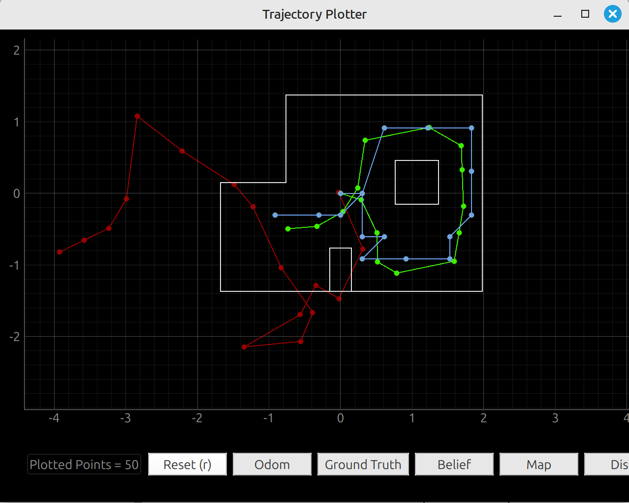
The first part of this lab was to download the required files to use the Bayes filter over Bluetooth. After downloading the files, I had to modify the perform_observation_loop function in the RealRobot class to communicate with my robot and have it send the ToF data. I edited the function to use the same code as my Lab 9 code for collecting mapping data. I also had to run the code in lab11_sim.ipynb to test the simulator again. This code is shown below, and is similar to Lab 10 in that the Bayes filter tracks the ground truth pretty well, but the odometry quickly gets lost.
Running the Bayes filter
With the code implemented, I was ready to start testing the Bayes filter. At first, I was getting very poor results, as shown in Figure 2. I tried debugging for a bit, but eventually concluded that it was the direction I was spinning. One of the bugs that I had during Lab 9 was that I spun my robot clockwise because that is the positive direction of the DMP, but the world frame is positive going counterclockwise. In Lab 9, I was able to fix this by just adding a - sign to my scans. However, that trick was still producing bad results. I ended up having to go back to my robot to make it rotate counterclockwise. This meant I had to add a bit of extra code to adjust the DMP output so it starts at 0° and increments counterclockwise. Normally, the DMP would count down from 360° when rotating counterclockwise. I also took 36 measurements, rather than the required 18. I was hoping that this would give me a better estimate.
case MAPPING_TURN: {
            float pid_percent = updatePID(mapping_pid);
            setBothMotors(pid_percent, -pid_percent); //Spin motors in oposite directions

            float yaw_error = mapping_pid.setpoint - yaw;
            if (yaw_error > 180.0f)  yaw_error -= 360.0f;
            if (yaw_error < -180.0f) yaw_error += 360.0f;
            if (fabs(yaw_error) < STEADY_STATE_THRESH_DEG) {
                if (steady_state_start_ms == 0) {
                    steady_state_start_ms = millis();
                } else if (millis() - steady_state_start_ms >= STEADY_STATE_DURATION_MS) {
                    steady_state_start_ms = 0;
                    brakeBothMotors(); // Stop both motors and make sure that robot has come to a complete stop
                    delay(50);
                    MappingState = MAPPING_COLLECT;
                }
            } else {
                steady_state_start_ms = 0; // reset if error spikes back up
                MappingState = MAPPING_TURN;
            }
            break;
        }

        case MAPPING_COLLECT: {
            int distance = getSensorDistance(distanceSensorFront);
            if (distance != -1){ // Valid measurement collected
                float normalized_yaw = start_yaw - yaw;
                if (normalized_yaw < 0.0f) normalized_yaw += 360.0f;
                map_data[points_collected].yaw = normalized_yaw;
                map_data[points_collected].distance = distance;

                setSetpoint(mapping_pid, start_yaw - points_collected * STEP_DEG);
                startPID(mapping_pid);
                points_collected++;
                if (points_collected >= MAPPING_POINTS) {
                    MappingState = MAPPING_END;
                    return;
                }
                MappingState = MAPPING_TURN;
            } else { // distance was bad
                MappingState = MAPPING_COLLECT;
            }
            break;
        }
Results
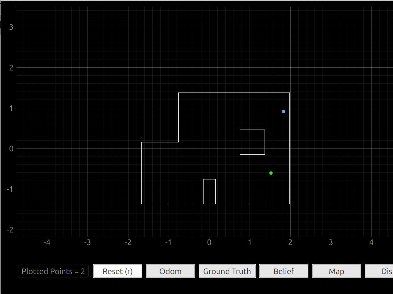
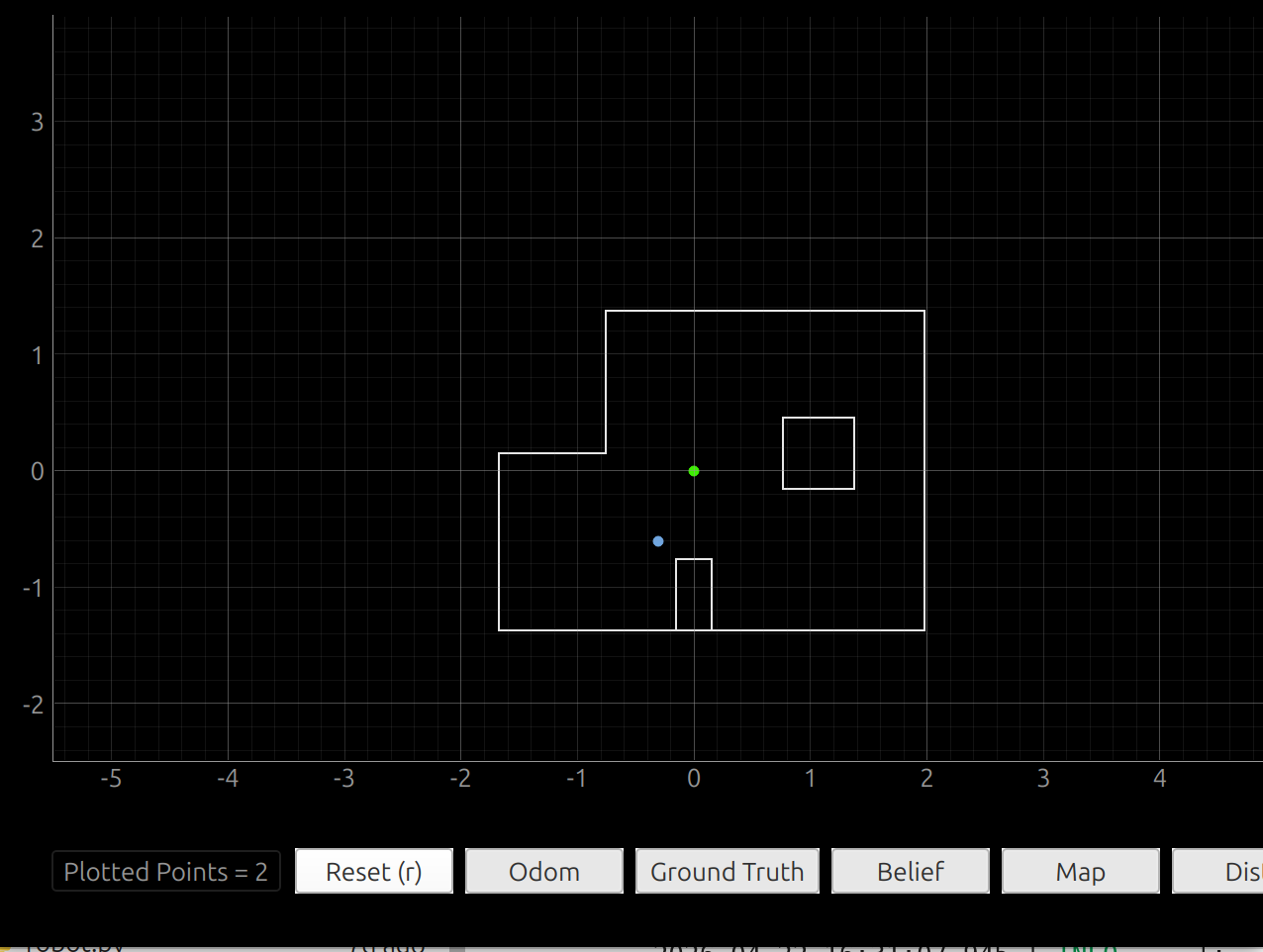
With the rotation aligned with the world, my results started to be reasonable. The green dot shows the actual position, while the blue dot shows the predicted position.
2026-04-22 16:31:07,937 | INFO |: Update Step
2026-04-22 16:31:07,945 | INFO |: | Update Time: 0.007 secs
2026-04-22 16:31:07,946 | INFO |: Bel index : (np.int64(4), np.int64(2), np.int64(5)) with prob = 1.0
2026-04-22 16:31:07,947 | INFO |: Bel_bar prob at index = 0.00051440329218107
2026-04-22 16:31:07,948 | INFO |: Belief : (-0.305, -0.610, -70.000)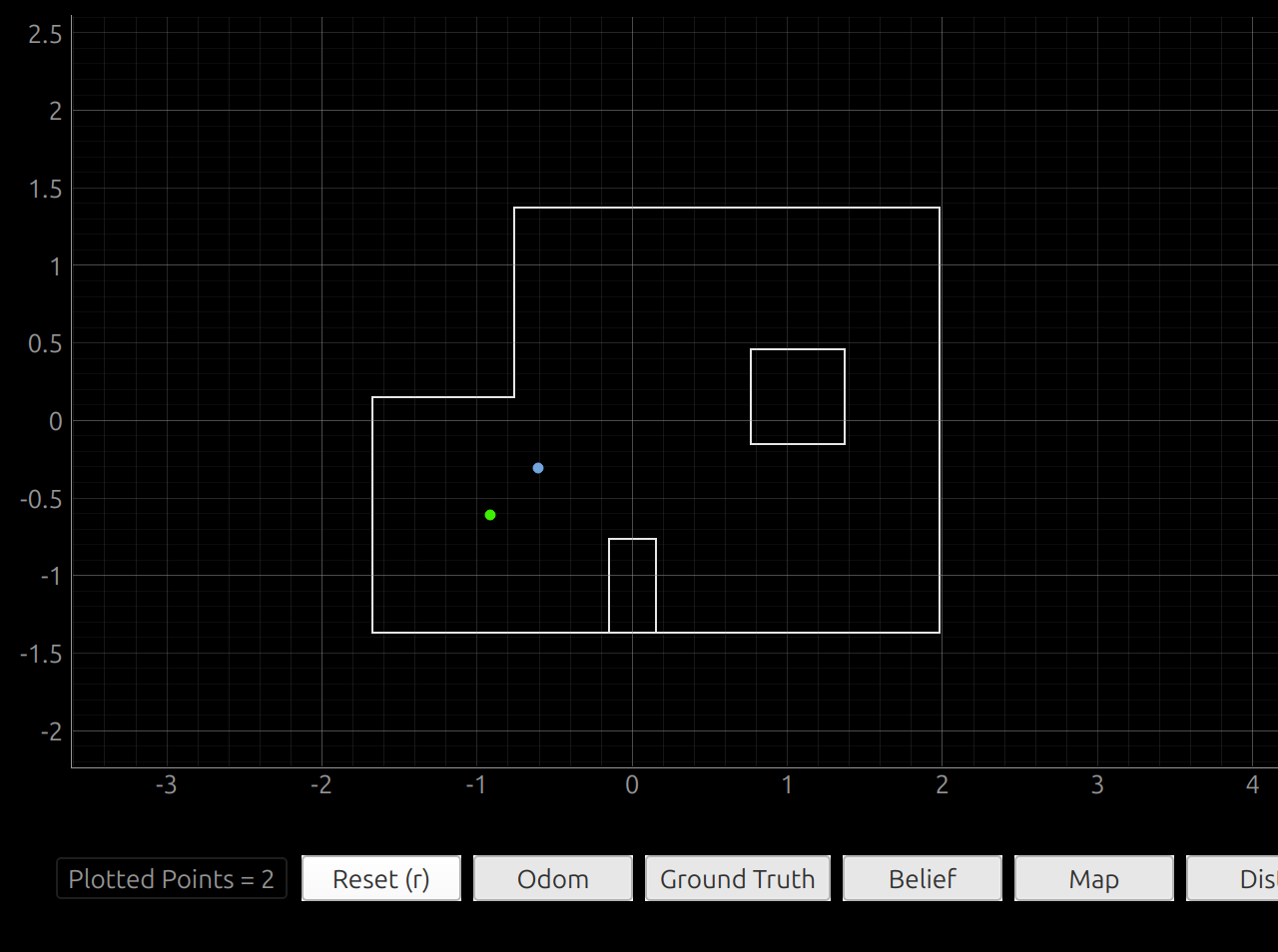
2026-04-22 16:51:25,218 | INFO |: Update Step
2026-04-22 16:51:25,223 | INFO |: | Update Time: 0.004 secs
2026-04-22 16:51:25,224 | INFO |: Bel index : (np.int64(3), np.int64(3), np.int64(7)) with prob = 1.0
2026-04-22 16:51:25,225 | INFO |: Bel_bar prob at index = 0.00051440329218107
2026-04-22 16:51:25,226 | INFO |: Belief : (-0.610, -0.305, -30.000)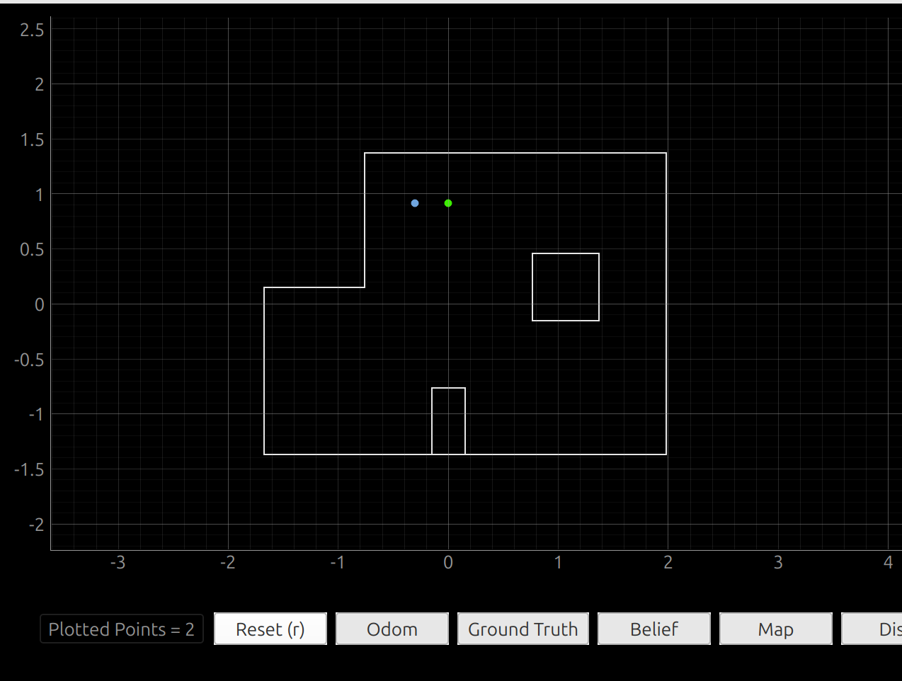
2026-04-22 16:44:17,385 | INFO |: Update Step
2026-04-22 16:44:17,388 | INFO |: | Update Time: 0.002 secs
2026-04-22 16:44:17,389 | INFO |: Bel index : (np.int64(4), np.int64(7), np.int64(7)) with prob = 0.9999999
2026-04-22 16:44:17,390 | INFO |: Bel_bar prob at index = 0.00051440329218107
2026-04-22 16:44:17,391 | INFO |: Belief : (-0.305, 0.914, -30.000)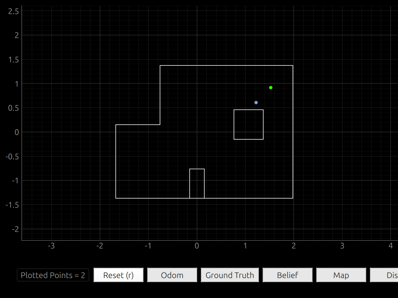
2026-04-22 16:47:55,038 | INFO |: Update Step
2026-04-22 16:47:55,041 | INFO |: | Update Time: 0.002 secs
2026-04-22 16:47:55,042 | INFO |: Bel index : (np.int64(9), np.int64(6), np.int64(6)) with prob = 1.0
2026-04-22 16:47:55,042 | INFO |: Bel_bar prob at index = 0.00051440329218107
2026-04-22 16:47:55,043 | INFO |: Belief : (1.219, 0.610, -50.000)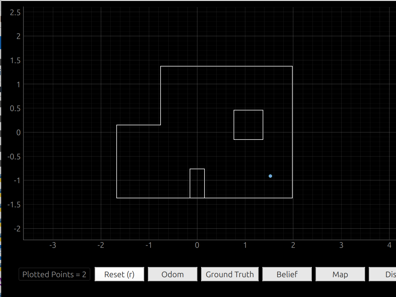
2026-04-22 16:38:55,580 | INFO |: Update Step
2026-04-22 16:38:55,583 | INFO |: | Update Time: 0.002 secs
2026-04-22 16:38:55,584 | INFO |: Bel index : (np.int64(10), np.int64(1), np.int64(7)) with prob = 1.0
2026-04-22 16:38:55,585 | INFO |: Bel_bar prob at index = 0.00051440329218107
2026-04-22 16:38:55,586 | INFO |: Belief : (1.524, -0.914, -30.000)
Looking at the results, we can see that most are not 100% accurate but are very confident in their positions. The 5, -3 scan was actually so perfect that it doesn’t show the actual dot, only the estimation. This scan is an outlier, though, since the rest of them are off by about 0.37 m on average. And all of them are very confident in their predictions. I used the default values from the Bayes filter. I should have set higher uncertainties for my sensors, since the results are clearly inaccurate, and being confidently wrong is not good behavior. I think that the reason the 5, -3 scan had such a good prediction was that it was in a very tightly packed area. But using this logic, 5, 3 should have also had better results, since it was up in the corner. I think that 5,3 didn’t do as well because of the larger gap to the west.
Acknowledgements
In this lab, I worked by myself, but I did discuss my results with Immanuel Koshy. I used AI to help convert my lab writeup from a Google Doc to Markdown.