Lab 3: ToF

Objective

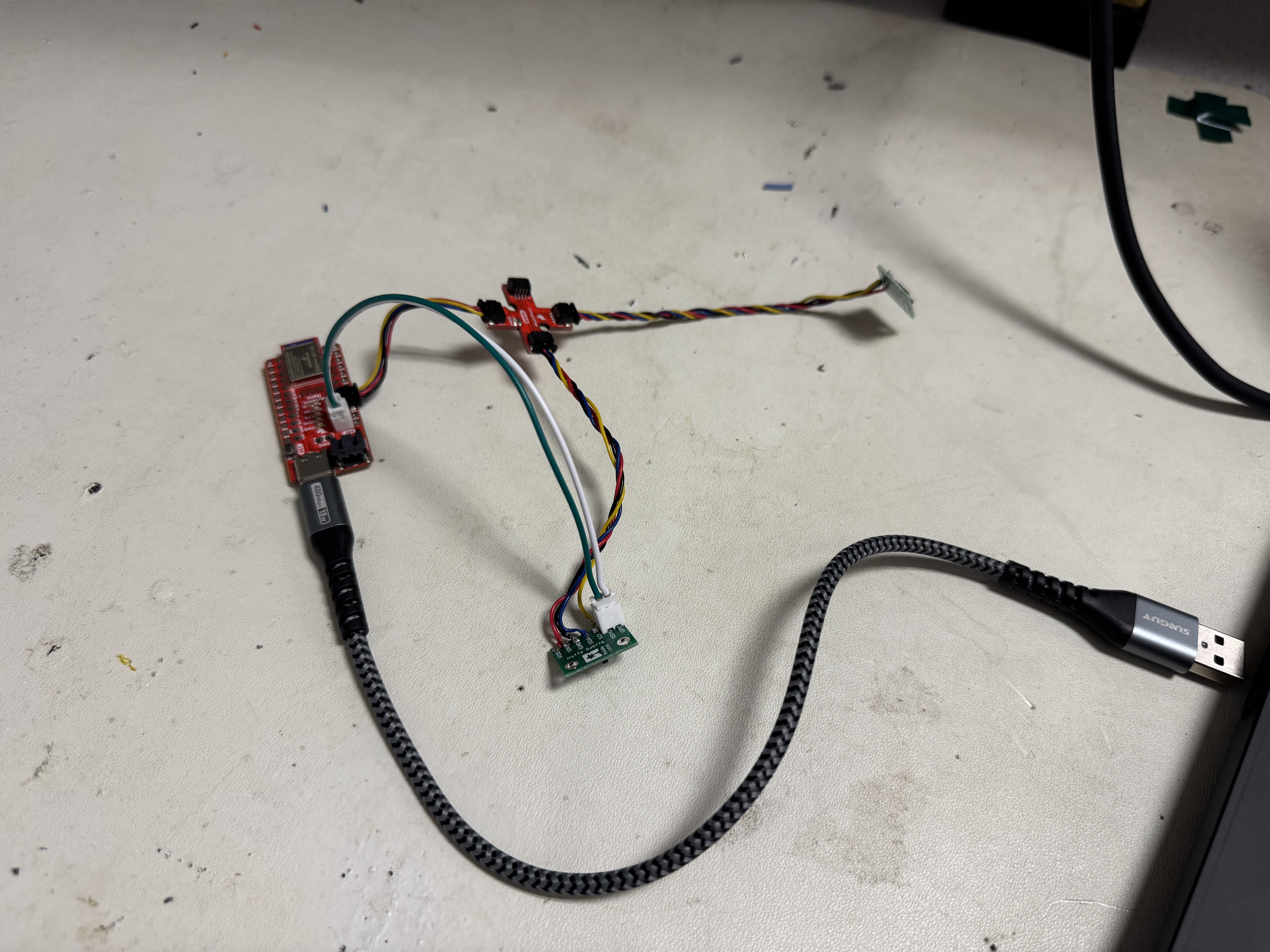
The objective of this lab was to connect two VL53L1X time of flight sensors to the Artemis, and transmit their distances over Bluetooth. To do this, we had to solder wires to the VL53L1X sensors because the versions that were provided did not have Qwiic connectors on them. This gave me the opportunity to practice my soldering.

Lab work

Prelab

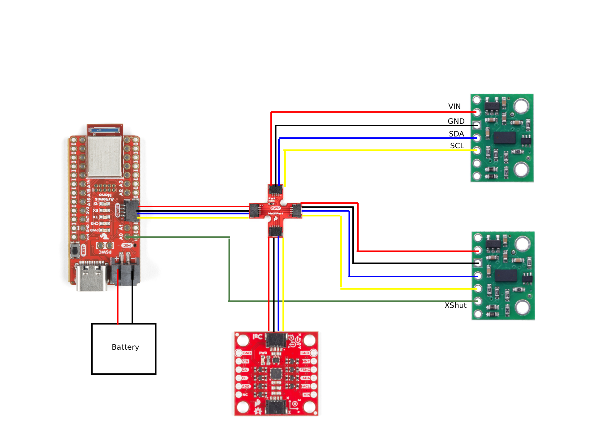
For the prelab, I had to think about the wiring of VL53L1X sensors. The VL53L1X has a quirk for its I²C address: it is hard coded on the sensor (0x29), but can be changed in software. This means that just connecting two sensors on the same I²C bus without changing one of the sensor’s addresses will cause both sensors to fail. To solve this problem, I soldered a JST connector to the Xshut pin on one of the sensors, and a JST connector to the Artemis. This is pictured in Figure 1. I chose to use a JST connector because I wanted the ability to easily remove the sensor, since it was connected via Qwiic already. I happened to have a kit of JST connectors lying around from another project, as well as a crimper so I could make my own cable.

With both sensors wired up, I was ready to write the software to connect them. To initialize both sensors, I set the GPIO connected to Xshut low to turn that sensor off, and then set the other sensor’s I²C address to 0x30. I checked to make sure that it worked, and then turned the original sensor on. This meant that the the sensors’ addresses ended up as 0x29 and 0x30.

pinMode(A0, OUTPUT); //Used to control xshut on the side ToF
digitalWrite(A0, LOW);  // Xshut low to set I2C address

sensor.setI2CAddress(0x30);

int tries = 0;
while((sensor.getI2CAddress() != 0x30) && (tries < SETUP_TRIES)){
    DEBUG_PRINTLN("Error setting I2C address");
    tries++;
}

if (tries >= SETUP_TRIES){
    return false;
}

digitalWrite(A0, HIGH);

With the sensors connected, I had to think about placement. I am going to place one sensor at the front of the car, and one on the right side. This will allow my car to follow walls, but only if the wall is on the right. I won’t be able to see anything on the left side of the car.

Lab

Battery

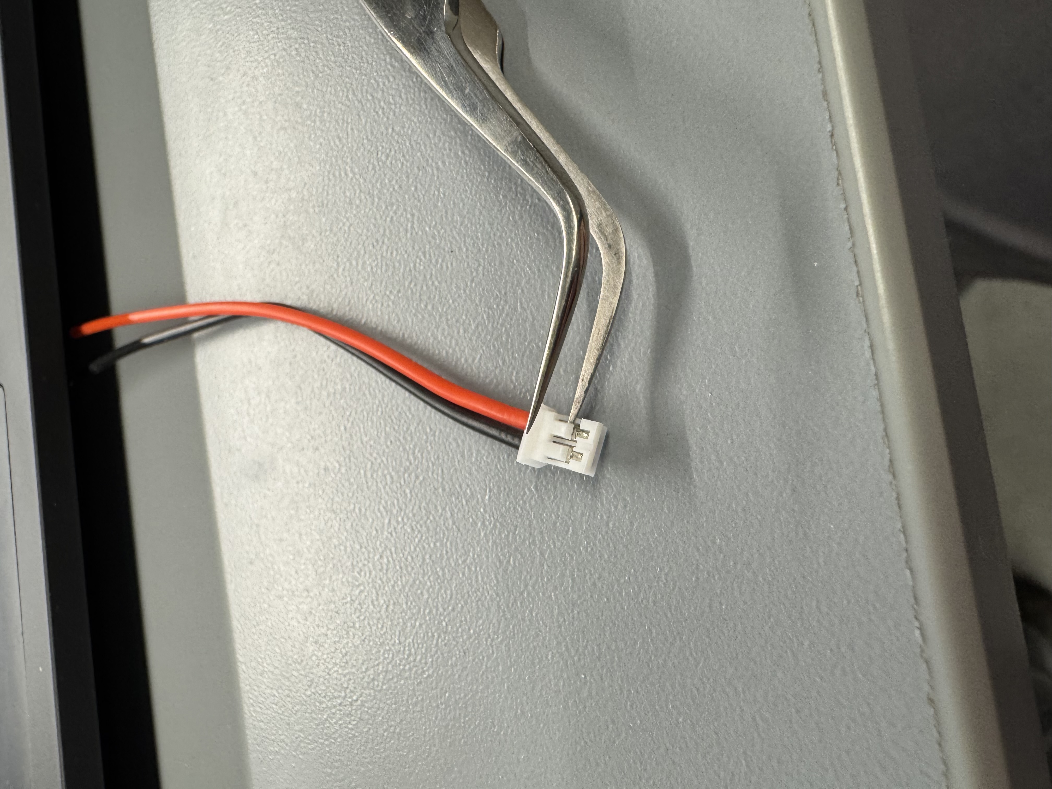
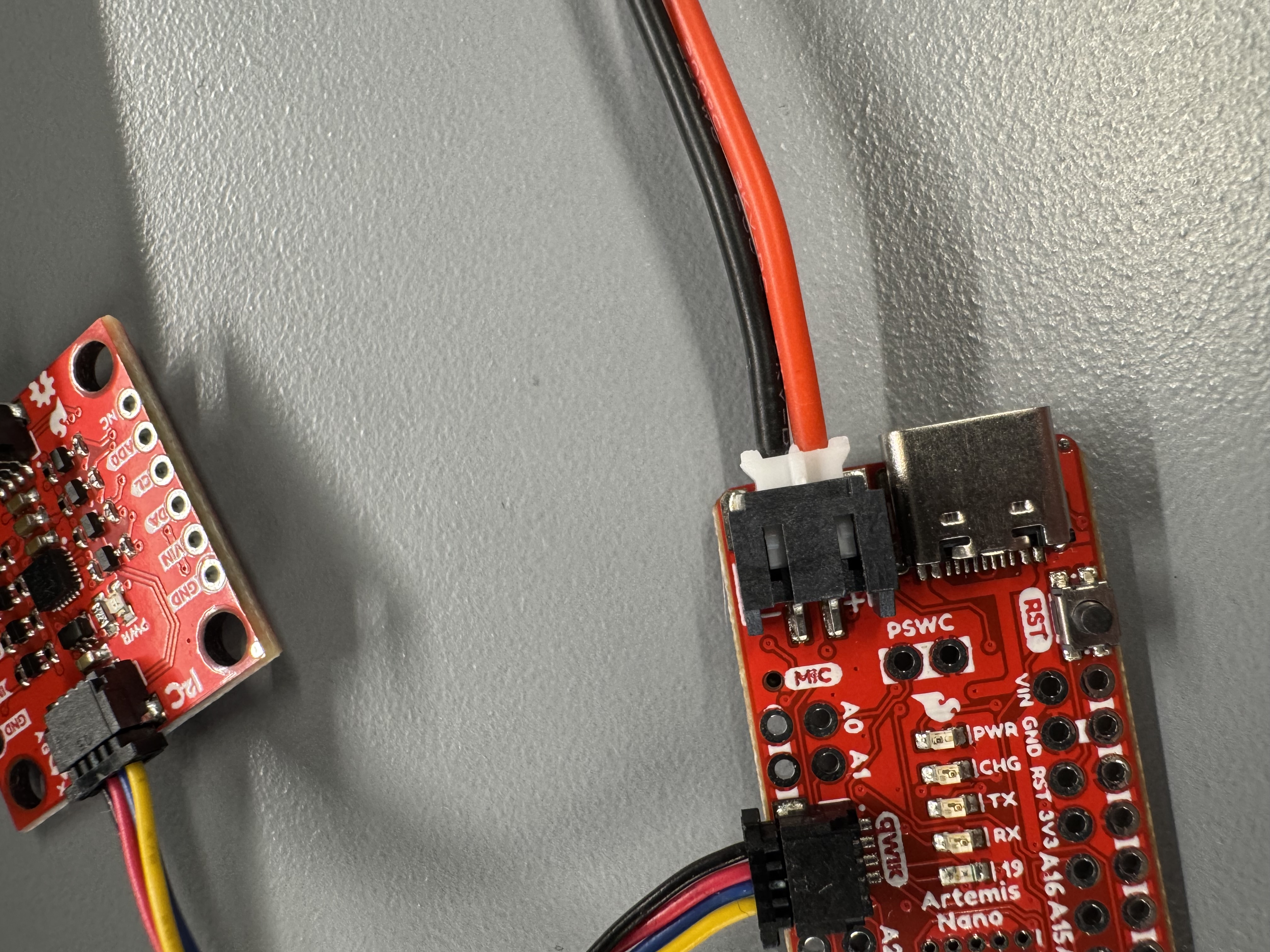
As part of this lab, we had to power the Artemis with a battery. Part of this included soldering a JST connector on the battery. The default JST polarity was inverted, so I would have had to solder the red battery lead to the black JST lead. This bothers me at a fundamental level, so I used a pair of tweezers to pull the wires out of the JST connector, and swapped them so all the wire colors matched. Figure 3 shows the swapping technique, and Figure 4 shows the polarity going into the Artemis.

ToF Software

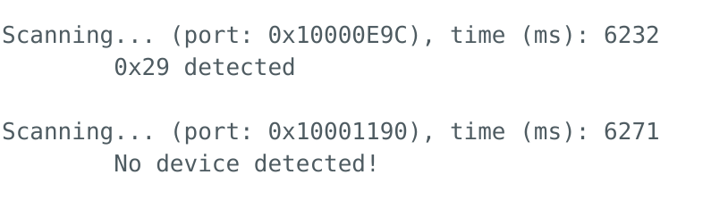
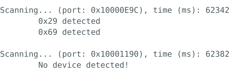
With the soldering done, it was time to start the software portion of the lab. First, I ran the build in Example05_wire_I2C which scans the I²C bus and prints the addresses of anything connected. I started by plugging in one ToF sensor, and the output is shown in Figure 5. It showed 0x29 as expected. I then plugged both ToF sensors in without changing the code at all. This is shown in Figure 6, and shows no addresses on the bus. Finally, Figure 7 shows one ToF sensor and the IMU to show that both sensors work when connected.

Sensor Accuracy

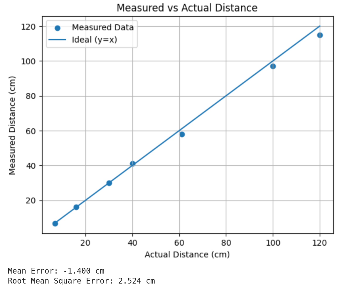
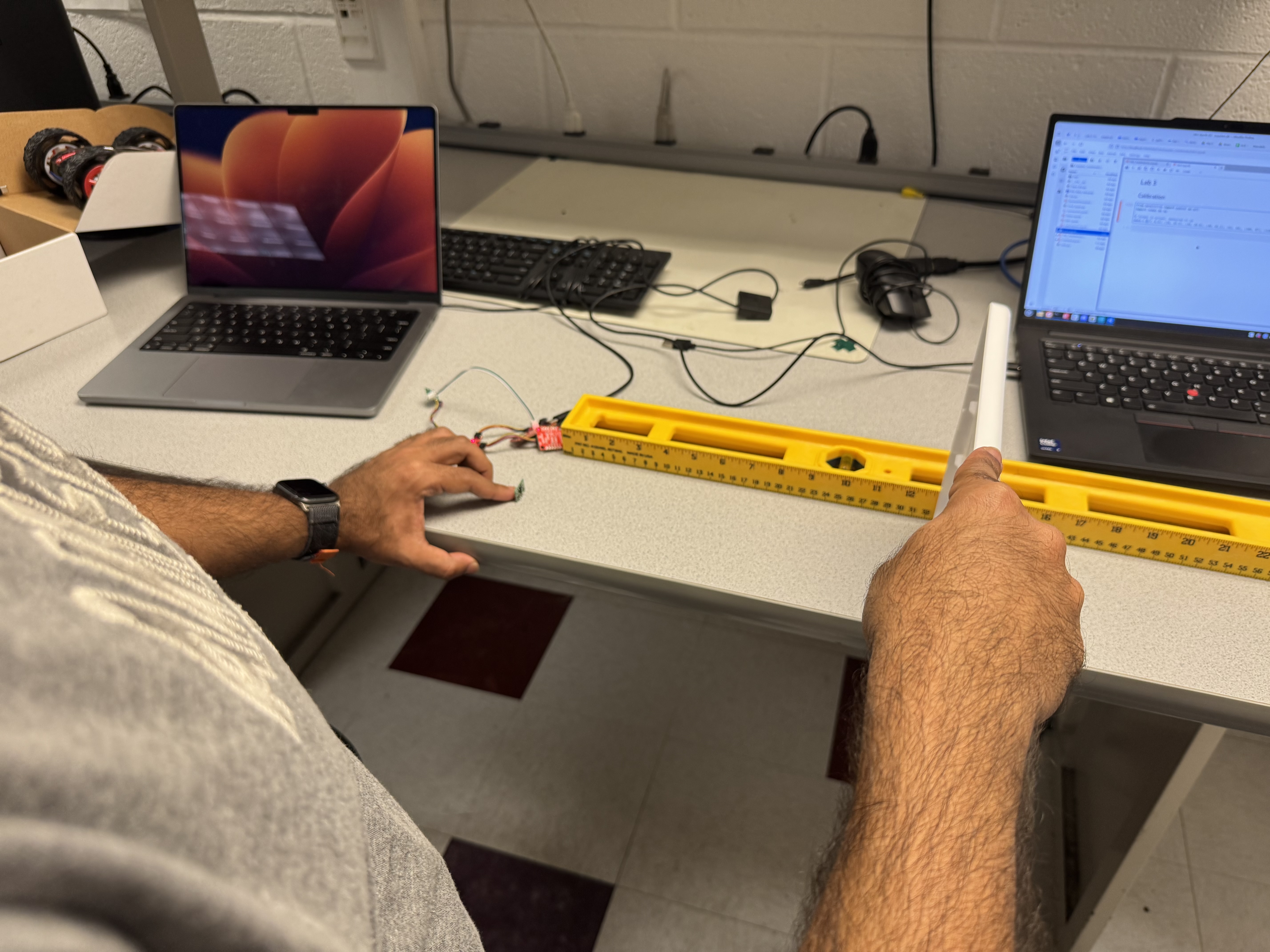
With the sensors working, I then had to test the accuracy of the sensor in one of the modes. I decided to use short mode, because I was working with Immanuel Koshy who was measuring long mode (See his page for his analysis). We had a large level with centimeters on it, and positioned the sensor at the end and used a storage bin lid at fixed distances and recorded the sensor measurement. The measurements are shown in Figure 8, and the setup is shown in Figure 9. I found that for the sensor I measured, it was very accurate at short distances, but at further distances it had a larger error. The average error of the sensor was -1.4 cm.

Sensor Speed

We want the microcontroller on the car to run as fast as possible. However, the way that the examples run the ToF sensor causes them to slow down by using a while loop to wait for data from the sensor, as shown in the code below.

void loop(){
  loop_count++;

  // --- Poll sensors, non-blocking ---
  if (distanceSensorFront.checkForDataReady()) {
    front_mm = distanceSensorFront.getDistance();   // consume new sample
    distanceSensorFront.clearInterrupt();           // ack/clear ready
    // If your library requires it: distanceSensorFront.startRanging();
    front_updates++;
  }

  if (distanceSensorSide.checkForDataReady()) {
    side_mm = distanceSensorSide.getDistance();
    distanceSensorSide.clearInterrupt();
    // If your library requires it: distanceSensorSide.startRanging();
    side_updates++;
  }

  // --- Periodic reporting (DO NOT print every iteration) ---
  uint32_t now = micros();
  if (now - last_report_us >= 100000) { // 100 ms
    float seconds = (now - last_report_us) / 1e6f;
    float loop_hz = loop_count / seconds;

    Serial.print("loop_hz=");
    Serial.print(loop_hz, 1);
    Serial.print(" front_hz=");
    Serial.print(front_updates / seconds, 1);
    Serial.print(" side_hz=");
    Serial.println(side_updates / seconds, 1);

    last_report_us = now;
    loop_count = 0;
    front_updates = 0;
    side_updates = 0;
  }
}

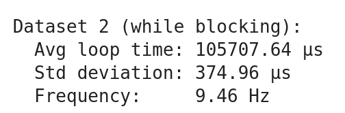
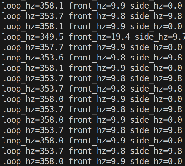
I ran a minimal test by printing the time since the last data was ready in a loop, and recorded that data. I tested both the while and if versions, and found that the frequency of the loop of each, shown in Figure 10. I found that the while version had a loop frequency of 9.46 Hz, while the non blocking version had a loop frequency of 224.27 Hz, a massive improvement. Both versions had a sensor frequency of around 10Hz. This makes sense because the Sparkfun VL53L1X has a timeout budget which is set to 100ms by default. The timing budget is what sets how long the sensor looks for a return signal. In the non-blocking version, the Serial prints is still probably what is limiting the speed, because Serial is slow.

loop_count++;

// --- Poll sensors, non-blocking ---
if (distanceSensorFront.checkForDataReady()) {
  front_mm = distanceSensorFront.getDistance();   // consume new sample
  distanceSensorFront.clearInterrupt();           // ack/clear ready
  // If your library requires it: distanceSensorFront.startRanging();
  front_updates++;
}

if (distanceSensorSide.checkForDataReady()) {
  side_mm = distanceSensorSide.getDistance();
  distanceSensorSide.clearInterrupt();
  // If your library requires it: distanceSensorSide.startRanging();
  side_updates++;
}

// --- Periodic reporting (DO NOT print every iteration) ---
uint32_t now = micros();
if (now - last_report_us >= 100000) { // 100 ms
  float seconds = (now - last_report_us) / 1e6f;
  float loop_hz = loop_count / seconds;

  Serial.print("loop_hz=");
  Serial.print(loop_hz, 1);
  Serial.print(" front_hz=");
  Serial.print(front_updates / seconds, 1);
  Serial.print(" side_hz=");
  Serial.println(side_updates / seconds, 1);

  last_report_us = now;
  loop_count = 0;
  front_updates = 0;
  side_updates = 0;
  }

ToF and IMU in parallel

Now that I had the ToF and IMU working, I had to think about how to collect data. The ToF sensors and IMU have different sample rates, and I need to make sure that the microcontroller runs fast, and none of the sensors block each other. To do this, I updated the IMU and ToF sensors independently each loop. This ensures that every sensor will be up to date. I also printed all the raw data from the ToF sensors and IMU over Serial and used SerialPlot to show them all working at the same time. The generated plot is very hard to read, but was all the data from the sensors. This is shown in the video below.

// Both called in loop()
bool imu_updated = updateIMU();

updateDistance(cur_dists, distanceSensorFront, distanceSensorSide);

// Collect data
if(recording){
    collectAllData(time_data, temp_data, imu_data, dist_data);
}

inline void updateDistance(Distances &out, SFEVL53L1X &frontSensor, SFEVL53L1X &sideSensor){

  if(frontSensor.checkForDataReady()){
    out.front = getSensorDistance(frontSensor);
  }

  if(sideSensor.checkForDataReady()){
    out.side = getSensorDistance(sideSensor);
  }
}

bool updateIMU(){
    unsigned long current_time = millis();
    float dt = (current_time - last_time) / 1000.0f; // Convert ms to seconds
    last_time = current_time;

    //IMU processing
    if (myICM.dataReady()) {
        comp_filter.dt = dt; // Update dt dynamically

        myICM.getAGMT();         // The values are only updated when you call 'getAGMT'

        updateGyroAttitude(&gyro_attitude, myICM, dt);
        updateAccelAttitude(&accel_attitude, myICM);

        updateCompFilter(&comp_filter, myICM, accel_attitude);
        return true;
    }
    return false;

}

ToF and IMU over Bluetooth

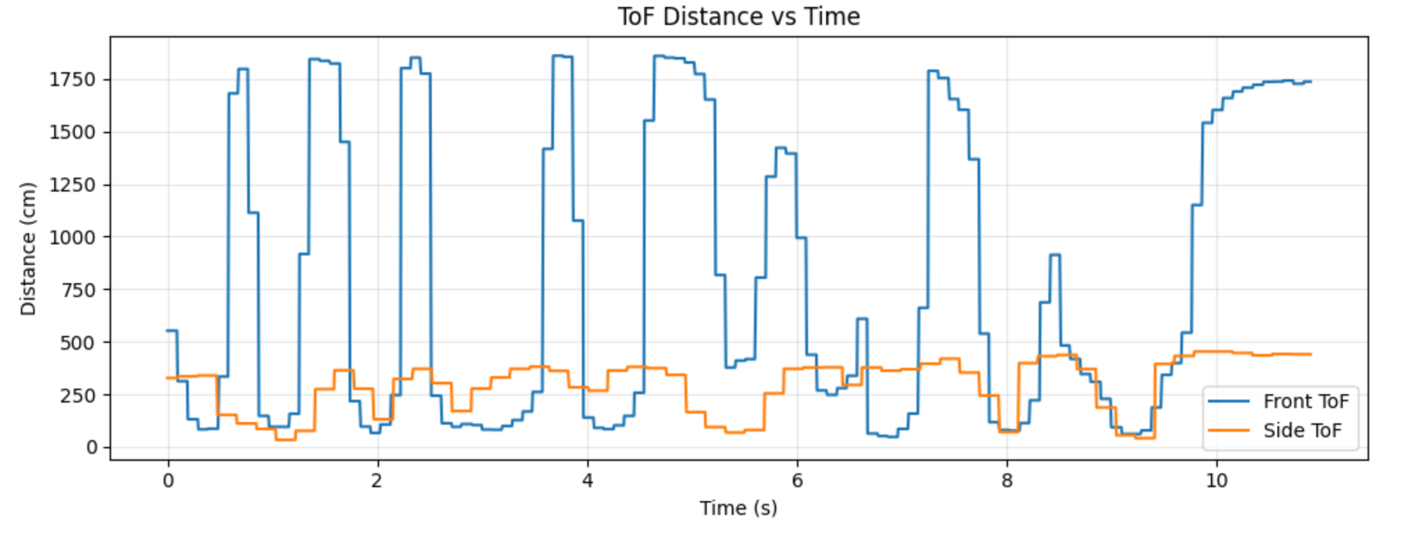
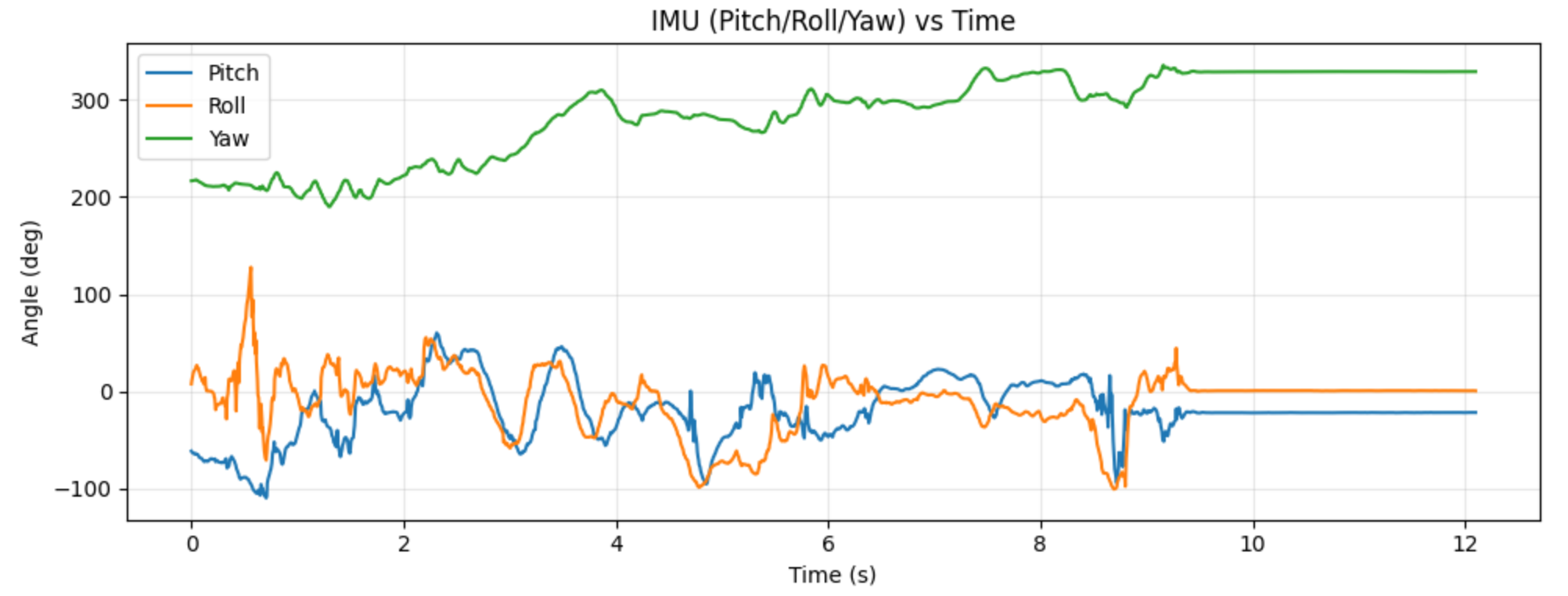
With both ToF sensors working, I had to store ToF data over time and send it to the Artemis via Bluetooth. I also sent IMU data to show that I could both. The graphs of each are shown in Figures 12 and 13. I sent about 12 seconds of data, and it probably took 30 because of how much data there was and how slow Bluetooth is. My current sending architecture is only suitable for logging data, not real time transmission.

Additional Tasks (5000-Level)

Infrared Sensors

In lecture we talked about many different types of infrared sensors. I will run through some of the pros and cons of each

• Amplitude IR Sensor

  • Pros
    • Cheap
    • Small
    • High sample rate (4kHz)
    • Simple circuit
  • Cons
    • Only works up to ~10 cm
    • Sensitive to ambient light, color, surface texture

  This sensor works by measuring the amplitude of the light emitted and then reflected.

• IR Triangulation Sensor

  • Pros
    • Simple circuit
    • Not sensitive to color, ambient light, or texture
    • Up to 1m range
  • Cons
    • Relatively expensive
    • Does not work in environments with high ambient light
    • Large
    • Low sample rate

This sensor works by bouncing light off of an object. It measures the angle of the light to determine the distance.

• Time of Flight IR Sensor
  • Pros
    • Very small
    • Not sensitive to color, ambient light, or texture
    • Highest range (up to 4m)
    • Largest dynamic range (0.1m - 4m)
  • Cons
    • Expensive
    • Complicated circuit
    • Low sample rate

This sensor works by emitting light, and then waiting for the light to return and measuring the time it took. It then can use the speed of light and time to calculate the distance.

• LiDAR Sensor
  • Pros
    • Can measure 3D environments
    • Measures reflectivity
    • Provides lots of data
  • Cons
    • Very expensive
    • More complicated to process data
    • Larger

Light Detection And Range (LiDAR) sensors are like ToF sensors, except instead of sending out a single beam they send out many. Mostly used on larger robots.

Color sensitivity

To test the sensors’ sensitivity to color and texture to color and texture, I grabbed an assortment of objects around my apartment. The sensor managed to detect all of the objects that I tested, which is a good sign. As discussed above, IR ToF sensors are not meant to be very sensitive to color and textures. Because they operate in the IR range (the VL53L1X emits light at 940 nm), the colors that humans can see shouldn’t impact the sensor much.

Collaborations

For this lab, I worked with Immanuel Koshy to measure our sensor accuracy. We helped each other by holding sensors and recording values. I used some AI for the Python plotting portions of this lab.