Lab 7: Kalman Filter

Objective

The objective of this lab was to develop a Kalman Filter, simulate it in Python, and then implement it on the car.

Lab work

Lab Tasks

Estimate Drag and Momentum

To implement the Kalman Filter, we first had to determine certain physical properties of the car for our model. Specifically, we needed to find the drag and momentum terms to use in our A and B matrices. To do this, I had to run the car towards the wall with a constant velocity, collecting data from the ToF sensor. To avoid hitting the wall, I couldn’t get my car to maintain a constant velocity. To fix this, I fitted an exponential function to the data to estimate the constant velocity. This initial work was done in Figure 1.

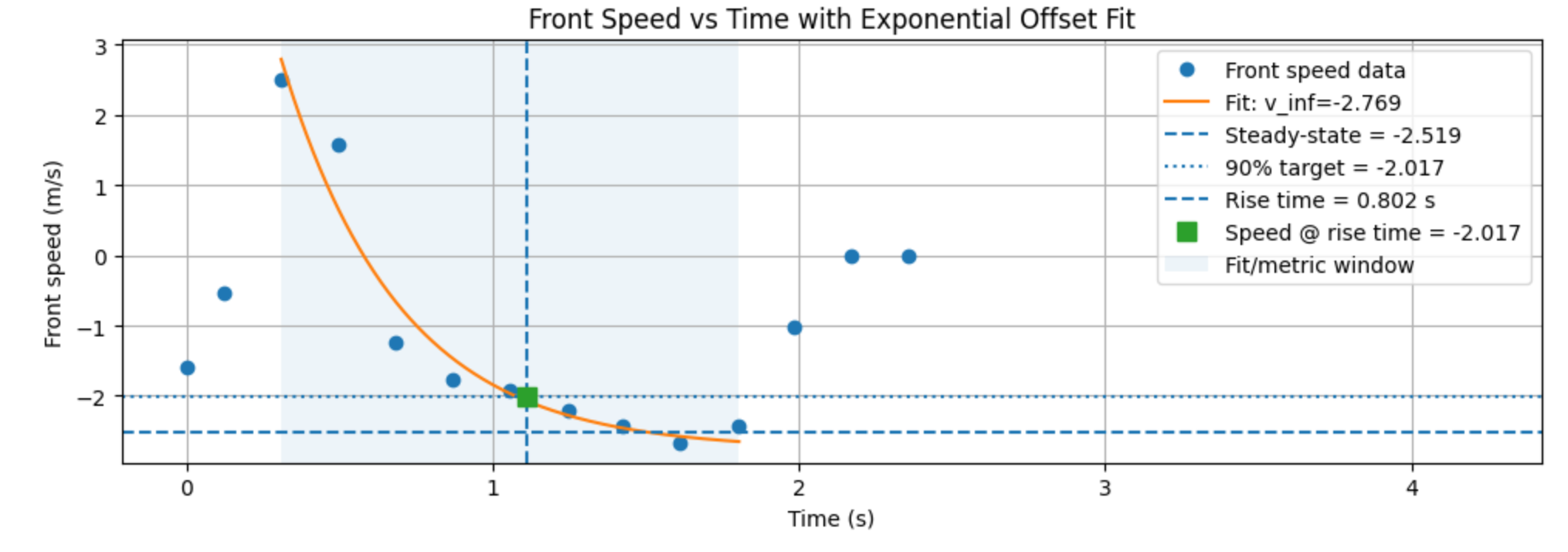
With the curve, I measured the steady state, 90% target, and rise time. With those values, I estimated d and m with the formulas:

$d = \frac{40}{|v_{ss}|}$

$m = \frac{-d \cdot t_r}{\ln(1 - 0.90)}$

I found that my d was 15.881127 and my m was 5.534828.

Kalman Filter in Python

With those determined, I set up my A and B matrices in Python, as well as C, my process noise and sensor noise. For my process noise, I started with 10mm for both the position and velocity uncertainties. These values should be small but nonzero, even though we know the car’s starting position is stationary. Using zero for either value will cause the filter to fail. For my measurement noise, I used 14mm, because in Lab 3, when I measured the accuracy of my ToF sensors, I found that it was 1.4cm/14mm. With all that data collected, I was ready to simulate the Kalman Filter in Python, which I did using the following code:

# ------------ d and m ----------------
d = 40 / abs(steady_state_speed)
m = (-d * rise_time) / math.log(1 - fraction)

print(f"d: {d:.6f}")
print(f"m: {m:.6f}")

# ------------ A and B -----------------
A = np.array([[0, 1],
              [0, -d/m]], dtype=float)

B = np.array([[0],
              [1/m]], dtype=float)

n = 2
Ad = np.eye(n) + ave_dt * A
Bd = ave_dt * B
C=np.array([[1,0]])
x = np.array([[data["front_dist"][0]],[0]]) # state vector

# -------------- Uncertainties ----------------

sigma_1 = (20 * 10**-3) * math.sqrt(ave_dt / 0.13)
sigma_2 = (10 * 10**-3) * math.sqrt(ave_dt / 0.13)
sigma_3 = 14*(10**-3) # 14mm measurement noise

sig_u=np.array([[sigma_1**2,0],[0,sigma_2**2]]) #We assume uncorrelated noise, and therefore a diagonal matrix works.
sig_z=np.array([[sigma_3**2]])

# -------------- Kalman Filter --------------------
def kf(mu,sigma,u,y):
    
    mu_p = Ad.dot(mu) + Bd.dot(u) 
    sigma_p = Ad.dot(sigma.dot(Ad.transpose())) + sig_u
    
    sigma_m = C.dot(sigma_p.dot(C.transpose())) + sig_z
    kkf_gain = sigma_p.dot(C.transpose().dot(np.linalg.inv(sigma_m)))

    y_m = y-C.dot(mu_p)
    mu = mu_p + kkf_gain.dot(y_m)    
    sigma=(np.eye(2)-kkf_gain.dot(C)).dot(sigma_p)

    return mu,sigma

mu = np.array([[data["front_dist"][0]],
               [0.05]], dtype=float)

sigma = np.array([[sigma_3**2, 0.0],
                  [0.0, 0.25**2]], dtype=float)

mu_kf = []
sigma_kf = []

for k, dist in enumerate(data["front_dist"]):
    u = np.array([[-data["right_motor"][k]]], dtype=float)
    y = np.array([[dist]], dtype=float)

    mu, sigma = kf(mu, sigma, u, y)

    mu_kf.append(mu.copy())
    sigma_kf.append(sigma.copy())


mu_kf = np.array(mu_kf).reshape(len(mu_kf), 2)

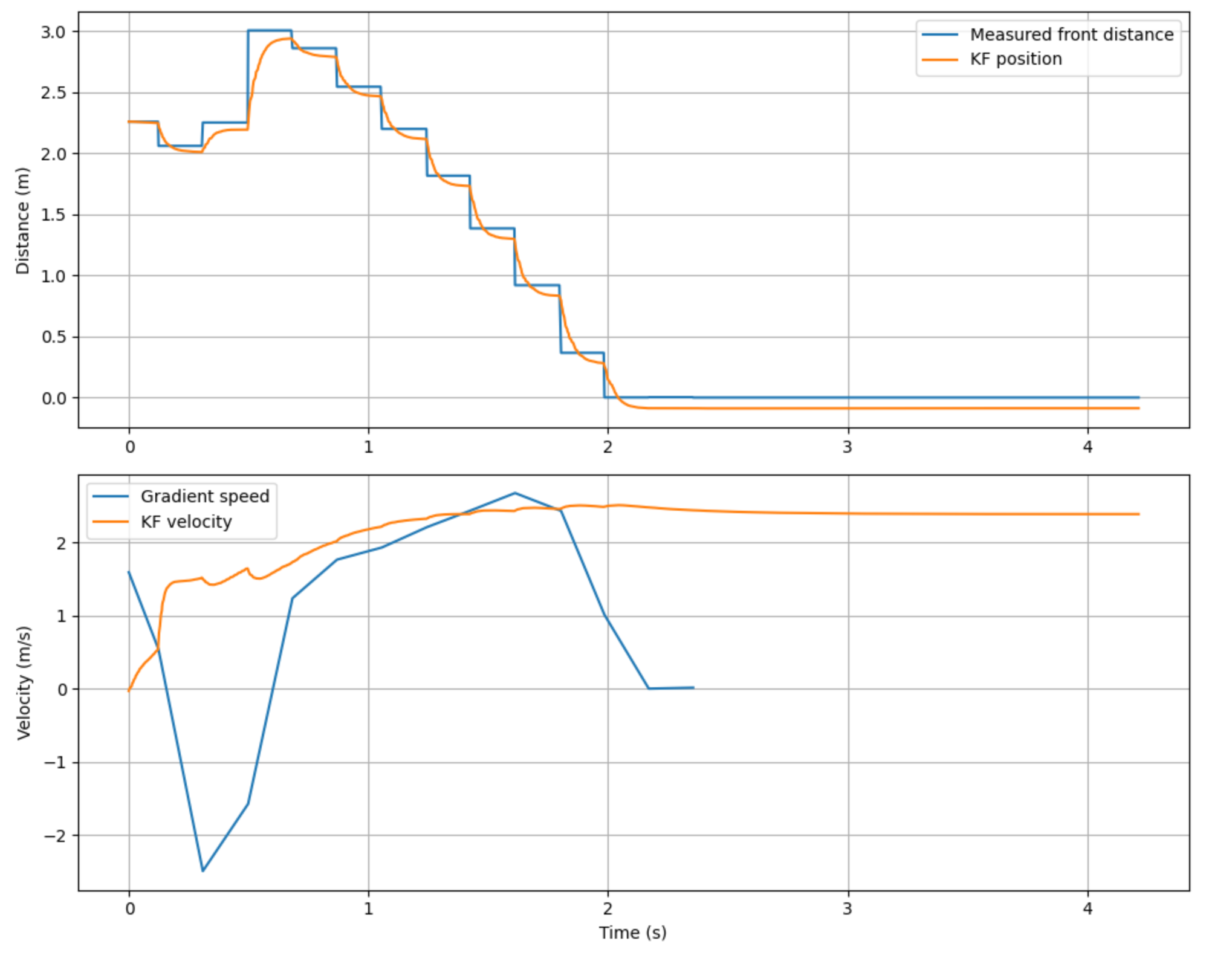
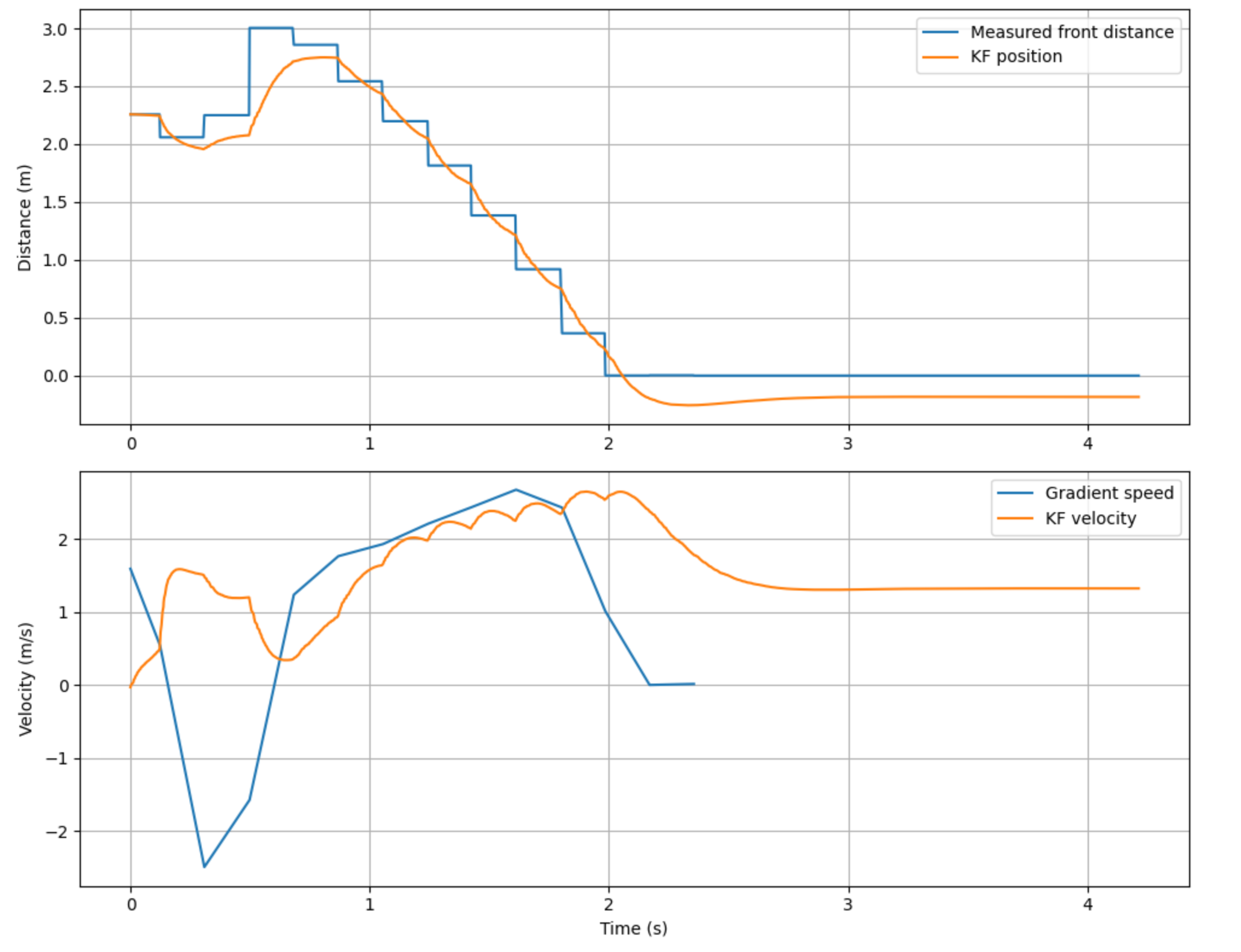
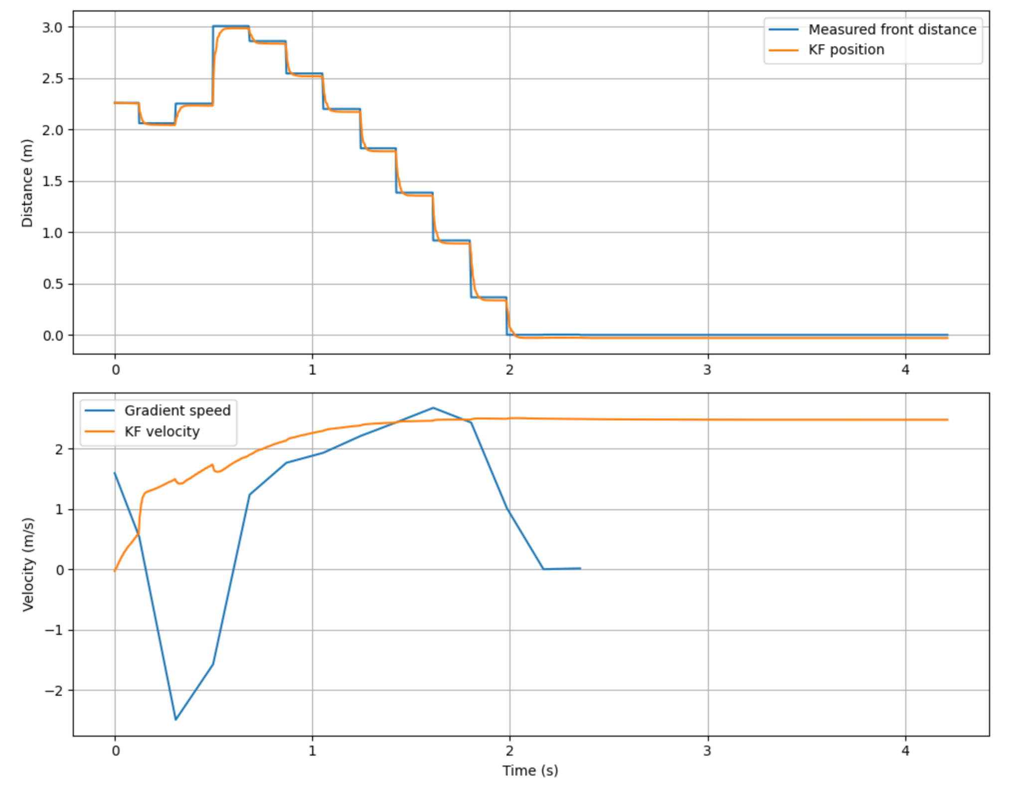
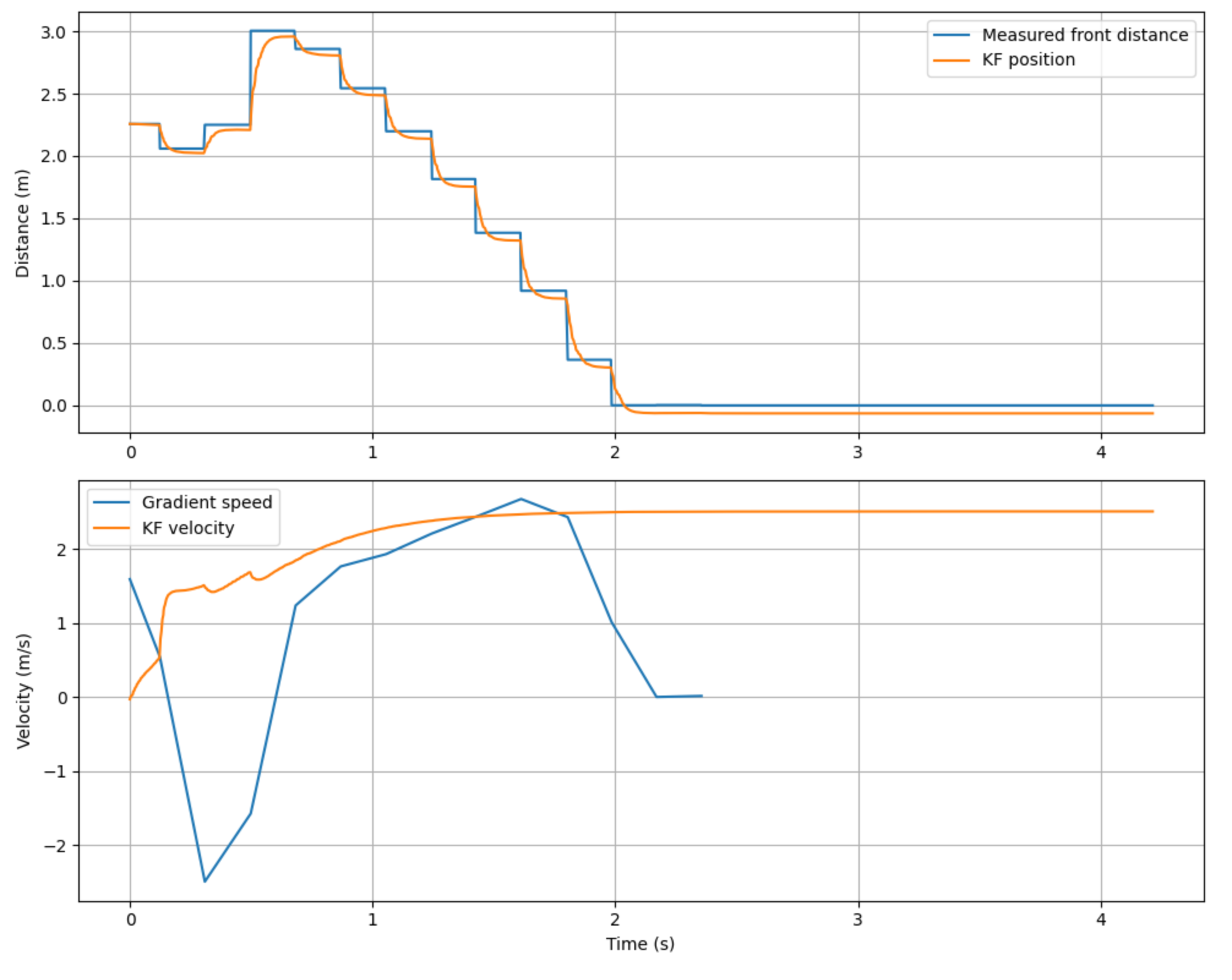
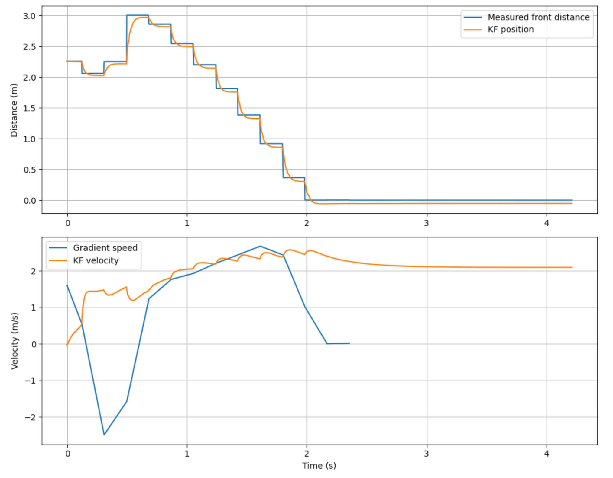
This code produced the graph of the Kalman filter vs. my example data shown in Figure 2. The position graph shows that the Kalman filter matches the time-of-flight data pretty well and looks much better than the simple linear predictions from Lab 5. We can see that the Kalman filter consistently estimates the car’s distance from the wall as greater than the ToF sensor’s when the ToF sensor updates. I found that increasing the sensor noise makes the filter adjust more slowly to jumps in distance caused by the ToF update, whereas smaller values produce steeper curves. I found that making sigma_1 smaller made the position curve look more linear and less like steps of exponential curves, as shown in Figure 3. Whereas making sigma_1 larger made the position graph match the ToF position, which was basically flat after the update step, as shown in Figure 4. Making sigma_2 smaller didn’t affect the position curve much, but it made the velocity curve smoother, as shown in Figure 5, whereas increasing sigma_2 added more jumps, as shown in Figure 6.

Kalman Filter on Robot

With the Kalman filter simulated in Python, it was time to implement it on my robot and integrate it into my system. I started by replicating the given Kalman filter code in C++ using the BasicLinearAlgebra library. This implementation is shown in Figure 7. I then edited my main to skip the linear prediction step and run the filter at each step, feeding it the PID controller’s output and ToF sensor reading. I also changed the PID controller to look at the Kalman Filter’s position output instead of the raw ToF sensor reading. I tried to improve performance by precomputing some process-noise values, but I recalculated dt on each loop to keep it more accurate. Arguably, I could use Python to calculate the loop speed and set dt to a constant to improve performance. I also tried to save a little bit of performance by inlining the kf() function. Although with how many other function calls that I have, its hard to say how much of a difference this makes.

inline void kf(Matrix<2, 1> &mu, Matrix<2, 2> &sigma, Matrix<1, 1> u, Matrix<1, 1> y) {
    
    // Time delta calculation
    static unsigned long kf_prev_time = micros();
    unsigned long current_time = micros();
    float dt = (current_time - kf_prev_time) / 1000000.0f; 
    dt = min(dt, 0.5f); // cap at 500ms to prevent blowup on first call
    kf_prev_time = current_time;

    // Dynamically calculate process noise variance
    float variance_step = (proc_noise / 0.13f) * dt; 
    Matrix<2, 2> sig_u = {variance_step, 0.0f,
                          0.0f, variance_step};

    // Dynamically construct discrete matrices
    Matrix<2, 2> Ad = {1.0f, dt,
                       0.0f, 1.0f - (dt * d / m)};

    Matrix<2, 1> Bd = {0.0f,
                       dt / m};

    // Prediction Step
    Matrix<2, 1> mu_p = Ad * mu + Bd * u;
    Matrix<2, 2> sigma_p = Ad * sigma * ~Ad + sig_u;
    
    // Measurement Update Step
    Matrix<1, 1> sigma_m = C * sigma_p * ~C + sig_z;
    Matrix<2, 1> kkf_gain = sigma_p * ~C * Inverse(sigma_m);
    
    Matrix<1, 1> y_m = y - C * mu_p;
    mu = mu_p + kkf_gain * y_m;
    sigma = (I - kkf_gain * C) * sigma_p;
    
}

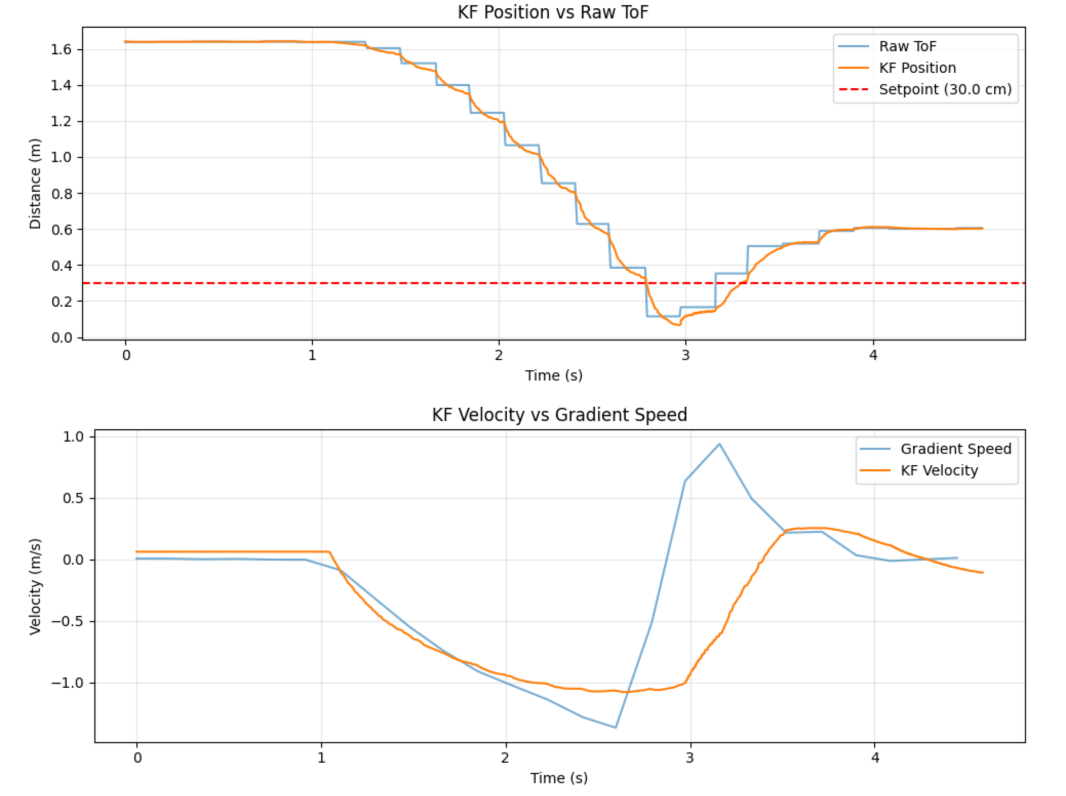
I found that the filter worked pretty well. My PID tuning got a bit messed up from changing the environment, but the filter predicts the distance pretty well. The filter’s performance is shown in Figure 8. It still tends to estimate the robot’s distance to the wall as greater than the ToF sensor initially, while approaching the wall. This is shown by the fact that when the ToF sensor updates, the sensor reading is lower than the Kalman Filter prediction. When moving away from the wall, the filter strongly thinks that the robot is closer to the wall than the ToF does. They do converge at the end when the robot is mostly stationary.

Collaborations

I talked with Immanuel Koshy about some high level content, but mostly worked on my own. I used AI to help format the writeup.