Lab 9: Mapping

Objective

The objective of this lab was to generate a map of a small space in the lab using the ToF sensor.

Lab work

Lab Tasks

Orientation Control

The first task of the lab was to collect data points at multiple locations on the map. To do this, I had to spin the car in a circle, taking ToF measurements at different yaws. Because I had previously set up multiple yaw PID controllers, I figured that I could easily use one for this task. I designed a simple state machine with 4 states: START, TURN, COLLECT, and END. The following state transition diagram shows the simplified behavior:

Here is the full state machine code:

switch(MappingState){
        case MAPPING_START:
            if(mapping_running){
                MappingState = MAPPING_COLLECT;
            } else {
                MappingState = MAPPING_START;
            }
            break;

        case MAPPING_TURN: {
            float pid_percent = updatePID(mapping_pid);
            setBothMotors(pid_percent, -pid_percent); //Spin motors in oposite directions

            float yaw_error = mapping_pid.setpoint - yaw;
            if (yaw_error > 180.0f)  yaw_error -= 360.0f;
            if (yaw_error < -180.0f) yaw_error += 360.0f;
            if (fabs(yaw_error) < STEADY_STATE_THRESH_DEG) {
                if (steady_state_start_ms == 0) {
                    steady_state_start_ms = millis();
                } else if (millis() - steady_state_start_ms >= STEADY_STATE_DURATION_MS) {
                    steady_state_start_ms = 0;
                    brakeBothMotors(); // Stop both motors and make sure that robot has come to a complete stop
                    delay(50);
                    MappingState = MAPPING_COLLECT;
                }
            } else {
                steady_state_start_ms = 0; // reset if error spikes back up
                MappingState = MAPPING_TURN;
            }
            break;
        }

        case MAPPING_COLLECT: {
            int distance = getSensorDistance(distanceSensorFront);
            if (distance != -1){ // Valid measurement collected
                map_data[points_collected].yaw = yaw; // use global yaw, already fresh from blocking loop
                map_data[points_collected].distance = distance;

                // Accumulate actual rotation with wrap handling
                float delta = yaw - prev_collect_yaw;
                if (delta > 180.0f)  delta -= 360.0f;
                if (delta < -180.0f) delta += 360.0f;
                accumulated_rotation += fabs(delta);
                prev_collect_yaw = yaw;

                setSetpoint(mapping_pid, yaw + 15); // Move in smaller increments to get more points
                startPID(mapping_pid);
                points_collected++;
                if (accumulated_rotation >= 360.0f || points_collected >= MAX_MAP_POINTS) {
                    MappingState = MAPPING_END;
                    return;
                }
                MappingState = MAPPING_TURN;
            } else { // distance was bad
                MappingState = MAPPING_COLLECT;
            }
            break;
        }

        case MAPPING_END:
            setBothMotors(0, 0);
            mapping_running = false;
            MappingState = MAPPING_START;
            break;
    }

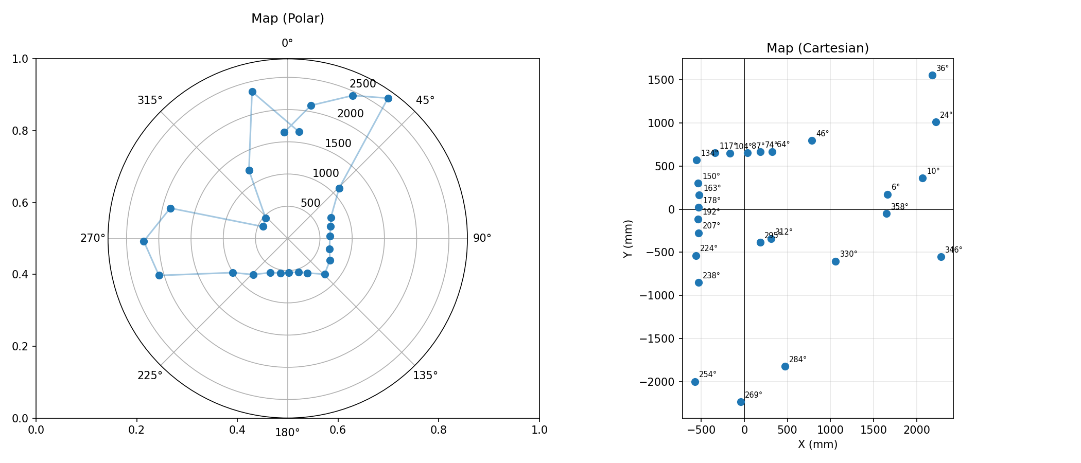
I did have to retune the PID controller a little bit to get good results. The lab required at least 14 points per scan with 20 degrees between them, but I collected more points and used smaller angles. I actually wish that I had collected even more points. But I found it really hard to get my robot to overcome static friction and start rotating without rotating too fast. I tried tapping my wheels, but that only helped a bit. Ultimately, I ended up with a more aggressive PID controller than I would have liked. The problem is that with very small motor inputs, only one side would actually spin, which caused the robot to translate, which is not good. Ultimately, I ended up with plots that look like this, which are ok but not perfectly accurate.

Here is a video of the robot taking a measurement:

Transformations

To combine the readings at each location into a single map, I had to perform transformations on them. The starting point is the sensor measurement $P_S$:

$P_S = \begin{bmatrix} d_i \\ 0 \\ 0 \\ 1 \end{bmatrix}$

This describes the sensor reading in the x-axis, zeros in all the other directions, and 1 as the homogeneous coordinate.

The first transformation that I did was the sensor to body frame. The ToF sensor is mounted at the front of my car, so it is not at the center of rotation. I measured that the ToF was about 8cm from the rough center of the car. The following transformation matrix performs this transformation by rotating the sensor by yaw and then offsetting the mounting distance.

${}^{B}T_S = \begin{bmatrix} \cos\theta_i & -\sin\theta_i & 0 & d_s\cos\theta_i \\ \sin\theta_i & \cos\theta_i & 0 & d_s\sin\theta_i \\ 0 & 0 & 1 & 0 \\ 0 & 0 & 0 & 1 \end{bmatrix}$

The next transformation is the body-to-world transformation. This translates the robot’s position into world space (using the known coordinates). Because I had already included the sensor rotation in the sensor-to-body transformation, the body-to-world matrix contains no rotation. You could put the rotation in either matrix, but not both. The actual matrix for body-to-world is:

${}^{W}T_B = \begin{bmatrix} 1 & 0 & 0 & x_r \\ 0 & 1 & 0 & y_r \\ 0 & 0 & 1 & 0 \\ 0 & 0 & 0 & 1 \end{bmatrix}$

To get the final output, we just need to multiply them together:

$P_W = {}^{W}T_B \cdot {}^{B}T_S \cdot P_S$

Which gives the following result:

$P_W = \begin{bmatrix} x_r + (d_s + d_i)\cos\theta_i \\ y_r + (d_s + d_i)\sin\theta_i \\ 0 \\ 1 \end{bmatrix}$

For my results, I had to make two corrections. The first is that I had to add a -90 degree offset to every yaw. I collected all my measurements with the robot facing directly south, so the IMU read it as 0°. But the world coordinate frame says that 0° is East. The second is that the DMP reports yaw increasing clockwise, but the world wants yaw increasing counterclockwise. So I had to sign flip all the yaws.

The following code implements the full transformation:

def transform_scan(df, tx_tiles, ty_tiles, yaw_offset_deg=0.0):
    x_r = tx_tiles * TILE_SIZE_M
    y_r = ty_tiles * TILE_SIZE_M
    # Global yaw offset goes into T_w_b
    T_w_b = pose_to_T(x_r, y_r, np.deg2rad(YAW_OFFSET_DEG))

    #Negative sign before df is from cw to ccw
    yaw_rad = np.deg2rad(-df['yaw_deg'].values + yaw_offset_deg)
    d_m     = df['distance_mm'].values / 1000.0
    N = len(d_m)

    pts_world = np.empty((N, 2))
    for i in range(N):
        T_b_s = T_rot_z(yaw_rad[i]) @ T_trans(SENSOR_OFFSET_M, 0)
        P_s   = np.array([d_m[i], 0.0, 0.0, 1.0])
        P_w   = T_w_b @ T_b_s @ P_s
        pts_world[i] = P_w[:2]
    return pts_world, (x_r, y_r)

Results

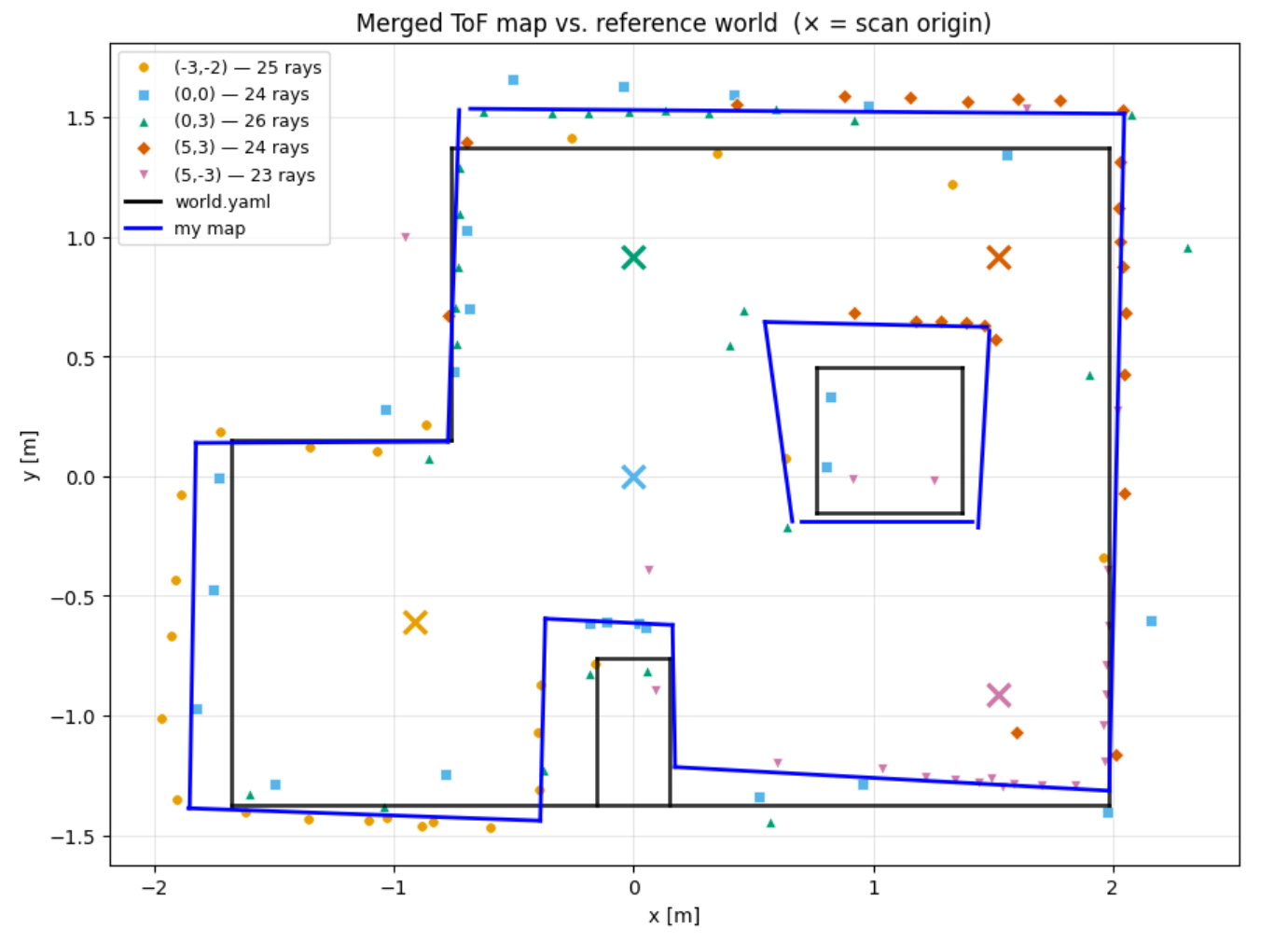
In the end, I was able to get a ok, but not perfect map. Figure 4 shows just my raw data points after the transformation.

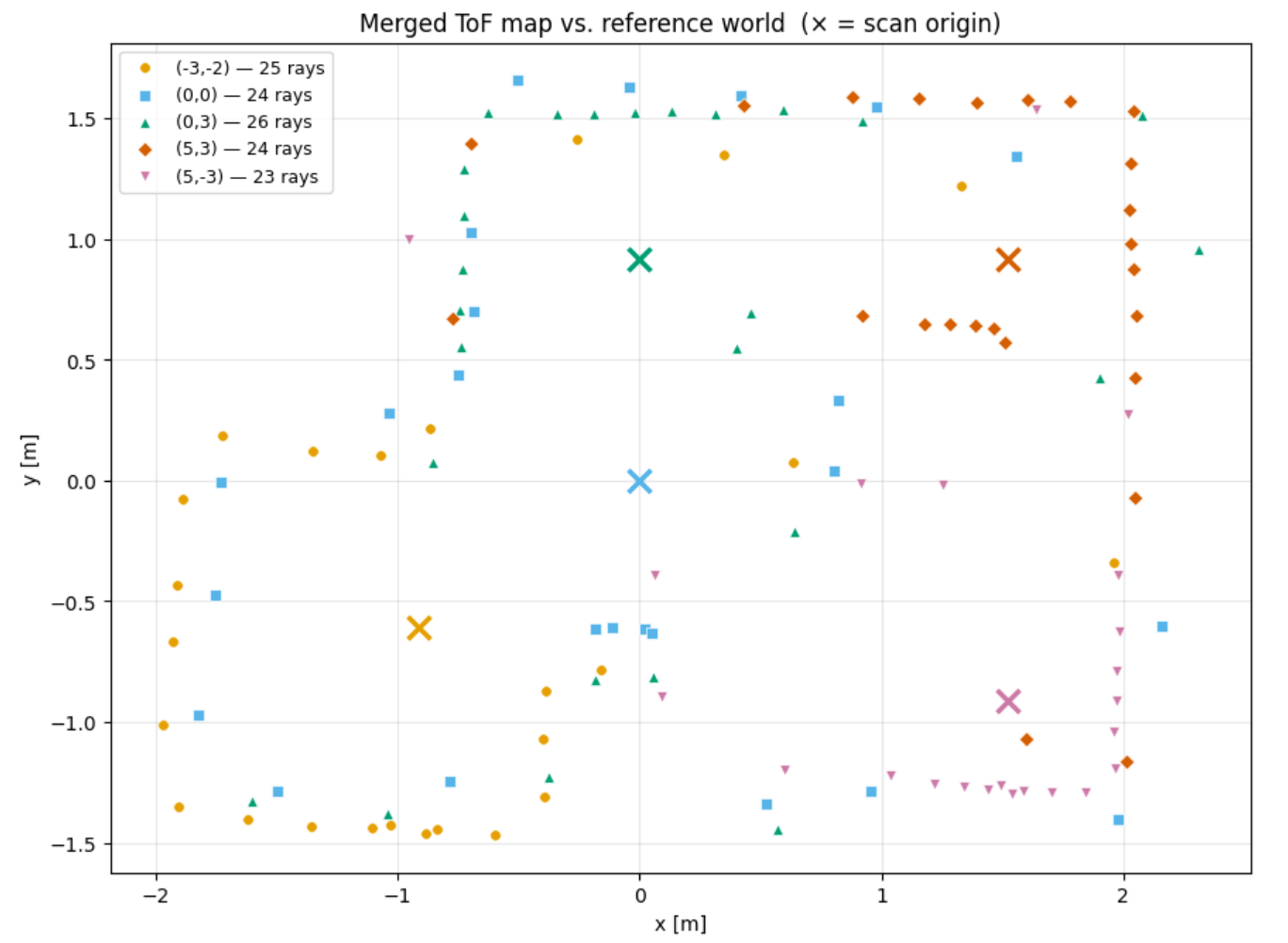
Figure 5 shows the actual world map overlaid on my points.

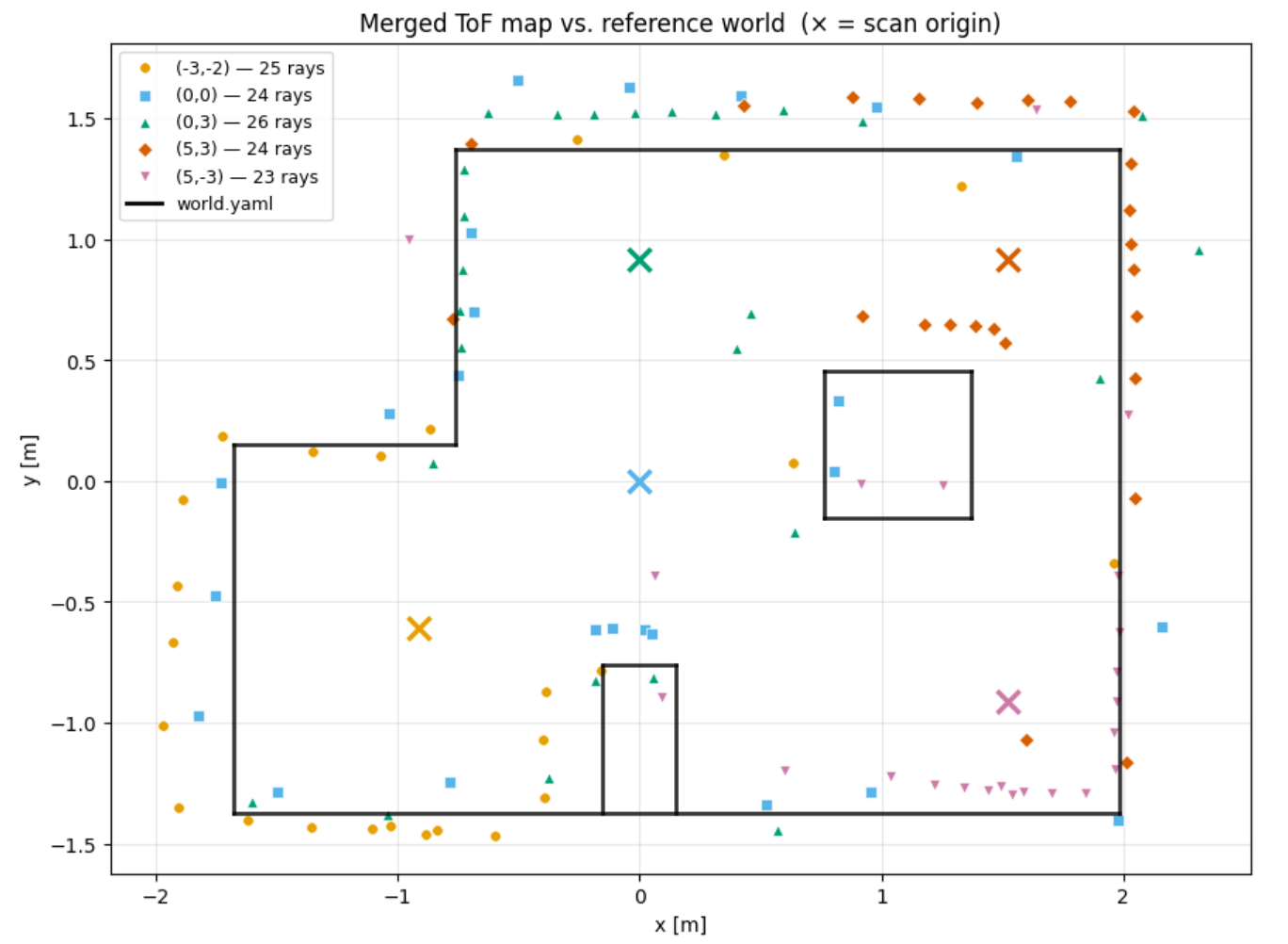
We can see that my scans missed some points on the south and east sides of the middle box, as well as the western side of the dent on the south. This is most likely caused by not collecting points at sufficiently small angle increments. Lots of the points were also collected as being further than they actually are. During the data collection, the car did translate a bit instead of only rotating around the point. This could cause some of the errors seen. I then placed points on the graph to generate the robot’s map. This is shown in Figure 6, and the points, my map, and world map are shown in Figure 7.

Overall, I am pleased with the results of my map, although I have some things to improve if I were to do it again.

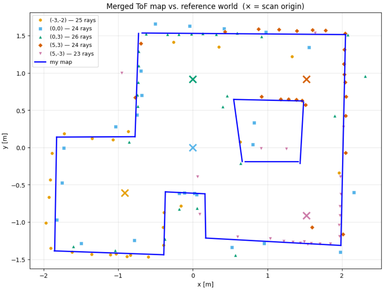
Overall, I am pleased with the results, although there are things I would improve if I were to do it again.

Acknowledgements

I talked a little bit with Immanuel Koshy about the high-level content of the lab, but I mostly worked alone.